Lecture 4: Lag Operator, MA Models, and AR Models

Raul Riva

FGV, Brazilian School of Economics and Finance (FGV EPGE)

October 2026

Econometrics I (Part I)

Introduction

Where We Are

• We will start covering a very useful modeling tool: ARMA models
• They combine autoregressive (AR) and moving average (MA) components
• In a certain sense, they are the most fundamental models for stationary time series
• There will be a neat theorem about this: Wold’s decomposition theorem (next lecture)

• But first we need to get acquainted with the lag operator \(L\)
• Never underestimate this guy!

The Lag Operator

Operators on Sequences

• An important vector space for us is the space of sequences
• Remember that time series are sequences of random variables

• An operator for us is a mapping from sequences to sequences
• The lag operator \(L\) shifts a sequence back by one period:

\[ L(y_t) = y_{t-1} \]

• This is an informal way of saying

\[ \{\cdots, y_{t-1}, y_t, y_{t+1}, \cdots\} \mapsto \{\cdots, y_{t-2}, y_{t-1}, y_t, \cdots\} \]

The Lag Operator Algebra

Some useful tricks:

• \(L(\alpha y_t) = \alpha y_{t-1} = \alpha L(y_t)\) for all \(\alpha \in \R\)
• \(L(y_t + z_t) = y_{t-1} + z_{t-1} = L(y_t) + L(z_t)\)
• It is a linear operator \(\implies\) all the machinery from functional analysis applies!

The most important property:

• \(L^2(y_t) = L(L(y_t)) = L(y_{t-1}) = y_{t-2}\)
• \(L^k(y_t) = y_{t-k}\) for any integer \(k > 0\)
• \(L^0(y_t) = y_t = I(y_t)\), the identity operator

The polynomial operator \(\phi(L) = a_0 I + a_1 L + a_2 L^2 + \dots + a_p L^p\) is such that \[ \phi(L)y_t = a_0 y_t + a_1 y_{t-1} + a_2 y_{t-2} + \dots + a_p y_{t-p} \]

Inverting Lag Polynomials

Can We Invert an Operator?

• Question: for a given operator \(T\), can we find an operator \(S\) such that \(ST = I\)?
• In other words, if I see \(T(y_t)\), can I recover the original sequence \(y_t\)?

• As you can imagine, this depends on the operator…
• Yes, you can invert the lag operator: \(L^{-1}(y_t) = y_{t+1}\)
• But not this one (dumb example): \(T(y_t) = 0\) \(\implies\) obviously you cannot invert it

It will be very useful to study the invertibility of the polynomials \(\phi(L)\):

• Let’s start with baby steps: assume \(\phi(L) = I - aL\) for some \(a \neq 0\)
• Challenge: can you invert this operator?

Can We Ever Invert \(\phi(L)\)?

• Inverting this operator means finding another operator \(\psi(L)\) such that \(\psi(L) \phi(L) = I\)
• Focus on scalar sequences, abuse notation, and write “1” instead of \(I\)
• If \(L\) were a number (it is not a number!!!), we would like to write \(\psi(L) = \frac{1}{1 - a L}\)
• If \(|aL| < 1\), we would be able to write \(\psi(L) = 1 + aL + a^2 L^2 + a^3 L^3 + \dots\)
• The problem with this intuition is that \(L\) is not a number!
• What does “\(|aL| < 1\)” even mean???

Truncating the Series

• Let’s explore this intuition a bit more
• Consider \(\psi_n(L) = 1 + aL + a^2L^2 + \dots + a^n L^n\). Then

\[ \psi_n(L) \phi(L) = (1 + aL + a^2L^2 + \dots + a^n L^n)(1 - aL) = 1 - a^{n+1} L^{n+1} \]

Hence, \(\psi_n(L) \phi(L) y_t = y_t - a^{n+1} L^{n+1} y_t = y_t - a^{n+1} y_{t-n-1}\) for any sequence \(\{y_t\}_{t \in \mathbb{Z}}\).

• If \(|a| < 1\), then \(a^n \to 0\), and \(a^{n+1} y_{t-n-1}\) is probably very small
• For a stationary \(y_t\), \(a^{n+1} y_{t-n-1} \to 0\) in mean square (and almost surely)

• But if \(|a| \geq 1\), then \(a^{n+1} y_{t-n-1}\) never dies out!
• So, it seems that the invertibility of \(\phi(L)\) depends on the value of \(a\)…

A Tool from Functional Analysis

Theorem (Neumann Series; Lax (2002), Chapter 17, Theorem 2)

Let \(B\) be a Banach space and, for \(A: B \to B\), let \(\|A\| \equiv \sup_{\|x\| \leq 1} \|Ax\|\). If \(T: B \to B\) is a bounded linear operator and \(\|I - T\| < 1\), then \(T\) is invertible, with inverse \[ T^{-1} = \sum_{k=0}^{\infty} (I - T)^k \]

• Our Banach space: random sequences \(\{y_t\}_{t \in \mathbb{Z}}\) with \(\|y\| \equiv \sup_t \sqrt{\E[y_t^2]} < \infty\)
• Every weakly stationary process lives in it: \(\|y\| = \sqrt{\gamma_0 + \mu^2}\)
• \(L\) is linear and bounded: \(\|Ly\| = \sup_t \sqrt{\E[y_{t-1}^2]} = \|y\|\), so \(\|L\| = 1\)

In Our Example

• \(\phi(L) = I - aL\) is linear and bounded (why?)
• \(\|I - \phi(L)\| = \|I - I + aL\| = |a| \cdot \|L\| = |a|\)
• \(\|I - \phi(L)\| < 1 \iff |a| < 1\)

Now we use the theorem to get exactly what our intuition hinted at before: \[ \psi(L) \equiv \phi(L)^{-1} = \sum_{k=0}^{\infty} (aL)^k = I + aL + a^2 L^2 + a^3 L^3 + \dots \]

In terms of notation, everything below is equivalent:

• \(\phi(L)^{-1} \equiv \frac{1}{1 - aL} \equiv \frac{1}{\phi(L)}\)
• \(\frac{\phi_1(L)}{\phi_2(L)} \equiv \phi_1(L)\,\phi_2(L)^{-1}\): first invert \(\phi_2(L)\), then apply \(\phi_1(L)\)

What If \(|a| \geq 1\)?

• \(|a| > 1\): \(I - aL\) is still invertible! Write \(I - aL = -aL\,(I - a^{-1}L^{-1})\)
• The theorem applies to the second factor, since \(\|a^{-1}L^{-1}\| = 1/|a| < 1\)
• Exercise: show that \((I - aL)^{-1} = -\sum_{k=1}^{\infty} a^{-k} L^{-k}\) when \(|a| > 1\)
• But this inverse uses the future: \(y_{t+1}, y_{t+2}, \dots\)

• \(|a| = 1\): no inverse at all, since \(I - aL\) sends the bounded sequence \(y_t = a^t\) to zero

Convention

From now on, \(\phi(L)\) is invertible if its inverse is a power series in \(L\) only, so it only uses the past: \[ \phi(L)^{-1} = \sum_{k=0}^{\infty} \psi_k L^k \]

 

Questions?

Roots and the Unit Circle

A More Complicated Example

Let’s study a more complicated polynomial of order 2. Assume that \[ \phi(L) = I - a_1 L - a_2 L^2 \] What conditions on the parameters would imply invertibility?

Hint: what does the Fundamental Theorem of Algebra say about a polynomial of order \(p\), in general?

Every polynomial of order \(p\) has exactly \(p\) (maybe complex!) roots, counting multiplicity. So you can write \[ \phi(L) = \alpha\left(L - \lambda_1 I \right)\left(L - \lambda_2 I \right) = \left(\alpha \lambda_1 \lambda_2\right) \underbrace{\left(I - \frac{1}{\lambda_1} L\right)}_{\equiv\, \phi_1(L)}\underbrace{\left(I - \frac{1}{\lambda_2} L\right)}_{\equiv\, \phi_2(L)} \] for some (maybe complex) numbers \(\alpha\), \(\lambda_1\), and \(\lambda_2\).

Roots Outside the Unit Circle

• \(\phi_1(L)\) and \(\phi_2(L)\) are both invertible if and only if \(|\lambda_1| > 1\) and \(|\lambda_2| > 1\). Why?

• Now, let’s define \(\psi(L) \equiv \frac{1}{\alpha \lambda_1 \lambda_2} \phi_1(L)^{-1}\phi_2(L)^{-1}\)
• It’s clear that \(\psi(L) \phi(L) = I\). So, by definition, \(\psi(L) = \phi(L)^{-1}\)

• Conclusion: \(\phi(L)\) is invertible if and only if all its roots are outside the unit circle
• Just a fancy way of saying that the modulus of all roots must be strictly greater than 1
• This generalizes to polynomials of any order \(p\)

What to Do in Practice?

Given a polynomial \(\phi(L) = I - a_1 L - a_2 L^2 - \dots - a_p L^p\):

• Focus on its “sister polynomial” \(f(x) = 1 - a_1 x - a_2 x^2 - \dots - a_p x^p\)
• Find the roots of \(f\) (numerically, of course)
• Check the modulus of all roots: if they are all greater than 1, then \(\phi(L)\) is invertible

In Python:

• np.roots expects the coefficients from the highest power down: [-ap, ..., -a1, 1]
• statsmodels: ArmaProcess(ar=[1, -a1, ..., -ap]) has .arroots and .isstationary

 

Questions?

MA Models (Finally!)

The MA(q) Model

• A very important building block is the Moving Average (MA) model
• Let \(\varepsilon_t\) be a white noise process with zero mean and variance \(\sigma^2\)
• The MA model of order \(q\) is defined as

\[ y_t = \mu + \varepsilon_t + \theta_1 \varepsilon_{t-1} + \theta_2 \varepsilon_{t-2} + \dots + \theta_q \varepsilon_{t-q} = \mu + \sum_{i=0}^{q} \theta_i \varepsilon_{t-i} \] where \(\mu\) is the mean of the process and the \(\theta_i\)’s are the parameters of the model (\(\theta_0 \equiv 1\)).

• This is a tool to model dependence that will completely die after \(q\) periods!

Notice we can write \(y_t = \mu + \theta(L) \varepsilon_t\), where \(\theta(L) = 1 + \theta_1 L + \theta_2 L^2 + \dots + \theta_q L^q\).

Is the MA(q) Stationary?

• The mean: \(\E[y_t] = \mu + \E[\varepsilon_t] + \sum_{i=1}^{q} \theta_i \E[\varepsilon_{t-i}] = \mu\)
• The variance (shocks are uncorrelated): \(\Var(y_t) = \sum_{i=0}^{q} \theta_i^2 \sigma^2 = \sigma^2\left(1 + \sum_{i=1}^{q} \theta_i^2\right)\)
• What about autocovariances? What should \(\gamma_h \equiv \Cov(y_t, y_{t-h})\) be?

There will be two cases. First, let \(h > q\). Then \(\gamma_h = 0\). Why? What’s the intuition for this?

Now, what about \(h \leq q\)?

Let’s Do Simple Cases

If \(q=1\), then \(y_t - \mu = \varepsilon_t + \theta_1 \varepsilon_{t-1}\). Hence \[ \gamma_1 = \E[(y_t - \mu)(y_{t-1} - \mu)] = \E[(\varepsilon_t + \theta_1 \varepsilon_{t-1})(\varepsilon_{t-1} + \theta_1 \varepsilon_{t-2})] = \sigma^2\theta_1 \]

If \(q=2\), then \(y_t - \mu = \varepsilon_t + \theta_1 \varepsilon_{t-1} + \theta_2 \varepsilon_{t-2}\). Hence \[ \gamma_1 = \E[(\varepsilon_t + \theta_1 \varepsilon_{t-1} + \theta_2 \varepsilon_{t-2})(\varepsilon_{t-1} + \theta_1 \varepsilon_{t-2} + \theta_2 \varepsilon_{t-3})] = \sigma^2(\theta_1 + \theta_2\theta_1) \] and, very importantly, \(\gamma_2 \neq 0\) here as well: \[ \gamma_2 = \E[(\varepsilon_t + \theta_1 \varepsilon_{t-1} + \theta_2 \varepsilon_{t-2})(\varepsilon_{t-2} + \theta_1 \varepsilon_{t-3} + \theta_2 \varepsilon_{t-4})] = \sigma^2\theta_2 \]

General Case for \(\gamma_h\)

• If \(h \leq q\), then \(\gamma_h = \sigma^2 \sum_{i=0}^{q-h} \theta_i \theta_{i+h} = \sigma^2\left(\theta_h + \theta_1\theta_{h+1} + \dots + \theta_{q-h}\theta_q\right)\)
• If \(h > q\), then \(\gamma_h = 0\)

• True or false? “Any MA(q) is stationary”

• The case \(q = \infty\) is actually well-defined. In that case we write \(y_t = \mu + \sum_{i=0}^{\infty} \theta_i \varepsilon_{t-i}\)
• This is a stationary process as long as the variance of \(y_t\) is finite
• This is ensured by the following condition: \(\sum_{i=0}^{\infty} \theta_i^2 < \infty\)
• Under this condition, any MA(q) process, even with \(q=\infty\), is stationary!
• It’s also common to focus on autocorrelations, which are defined as \(\rho_h \equiv \gamma_h/\gamma_0\)

Dial the MA Coefficients

\(y_t = \varepsilon_t + \sum_{i=1}^{4} \theta_i \varepsilon_{t-i}\) with \(\varepsilon_t \iid N(0,1)\). The shocks stay fixed: only the \(\theta\)’s change

// Four sliders in a 2x2 grid. The theme's 190px label column is too wide
// for two columns, so each slider gets a narrow label and a shorter track.
viewof theta = Inputs.form(
  [-0.8, 0.5, 0.1, -0.2].map((v, i) =>
    Inputs.range([-1.5, 1.5], {value: v, step: 0.05, label: ["θ₁", "θ₂", "θ₃", "θ₄"][i], width: 400})),
  {template: inputs => {
    inputs.forEach(f => f.style.setProperty("--label-width", "50px"))
    return html`<div style="display: grid; grid-template-columns: auto auto; justify-content: center; column-gap: 60px">${inputs}</div>`
  }}
)

maShocks = {
  const draw = d3.randomNormal.source(d3.randomLcg(2026))(0, 1)
  return Float64Array.from({length: 304}, draw)
}

// theta_0 = 1, then the four slider values
maCoefs = [1, ...theta]

// y_t = sum_i theta_i e_{t-i}
maPath = d3.range(4, maShocks.length).map(t => ({
  t: t - 3,
  y: d3.sum(maCoefs, (c, i) => c * maShocks[t - i])
}))

// gamma_h / sigma^2 = sum_i theta_i theta_{i+h}, which is zero for h > 4
maGamma = h => d3.sum(maCoefs.slice(0, Math.max(maCoefs.length - h, 0)), (c, i) => c * maCoefs[i + h])
maACF = d3.range(13).map(h => ({h, rho: maGamma(h) / maGamma(0)}))

// q = index of the last nonzero theta (0 means white noise)
maQ = d3.max(maCoefs.map((c, i) => (c !== 0 ? i : 0)))

maPanel = (title, plot) => html`<div>
  <div style="text-align: center">${title}</div>
  ${plot}
</div>`

html`<div style="display: flex; gap: 20px; justify-content: center; font-size: 19px">
${maPanel(html`One path, Var(<i>y<sub>t</sub></i>) = ${maGamma(0).toFixed(2)}`, Plot.plot({
  width: 590, height: 380, marginLeft: 50, marginBottom: 45,
  style: {fontSize: "18px", fontFamily: "Arial, Arimo, sans-serif"},
  x: {label: "Periods", labelAnchor: "center", labelArrow: "none"},
  y: {label: null, domain: [-6, 6], ticks: 5},
  grid: true,
  marks: [
    Plot.ruleY([0], {stroke: "black", strokeDasharray: "5,4"}),
    Plot.line(maPath, {x: "t", y: "y", stroke: "#0072BC", strokeWidth: 1.3, clip: true})
  ]
}))}
${maPanel(html`Autocorrelation <i>ρ<sub>h</sub></i>, <i>ρ</i><sub>1</sub> = ${maACF[1].rho.toFixed(2)}`, Plot.plot({
  width: 590, height: 380, marginLeft: 50, marginBottom: 45,
  style: {fontSize: "18px", fontFamily: "Arial, Arimo, sans-serif"},
  x: {label: "Lag h", domain: [-0.5, 12.5], ticks: d3.range(0, 13, 2), labelAnchor: "center", labelArrow: "none"},
  y: {label: null, domain: [-1, 1], ticks: 5},
  grid: true,
  marks: [
    Plot.ruleY([0], {stroke: "black"}),
    Plot.ruleX([maQ + 0.5], {stroke: "#EB811B", strokeWidth: 2, strokeDasharray: "7,5"}),
    Plot.ruleX(maACF, {x: "h", y1: 0, y2: "rho", stroke: "#0072BC", strokeWidth: 2.5}),
    Plot.dot(maACF, {x: "h", y: "rho", fill: "#0072BC", r: 5}),
    Plot.text([maQ === 0 ? "white noise: ρ = 0 at every lag h ≥ 1" : `ρ = 0 at every lag h > q = ${maQ}`], {frameAnchor: "top-right", dx: -10, dy: 10, fill: "#EB811B", fontWeight: "bold", fontSize: 20, stroke: "white", strokeWidth: 6})
  ]
}))}
</div>`

AR Models

The AR(p) Model

• The MA-type dependence might not be suitable for all time series data
• Example: effects of shocks might be long-lasting and never completely die out
• In such cases, we can use Autoregressive (AR) models

An AR(\(p\)) process satisfies the following dynamics: \[ y_t = \mu + \phi_1 y_{t-1} + \phi_2 y_{t-2} + \dots + \phi_p y_{t-p} + \varepsilon_t \]

In lag operator notation:

\[ y_t = \mu + \sum_{i=1}^{p} \phi_i L^i y_t + \varepsilon_t \implies \left(1 - \sum_{i=1}^{p} \phi_i L^i\right) y_t = \mu + \varepsilon_t \implies \Phi(L) y_t = \mu + \varepsilon_t \]

where \(\Phi(L) \equiv I - \sum_{i=1}^{p} \phi_i L^i\).

Is the AR(p) Stationary?

• At this point, we are already good friends with \(\Phi(L)\)
• This is the same type of polynomial we talked about!
• What are the conditions for the invertibility of \(\Phi(L)\)?

• The roots of \(f(x) = 1 - \phi_1 x - \phi_2 x^2 - \dots - \phi_p x^p\) should lie outside the unit circle
• If we can invert \(\Phi(L)\), we already know that \(\Phi(L)^{-1}\) has infinitely many terms
• If \(\Phi(L)^{-1}\) exists, we can write \(y_t = \Phi(L)^{-1}\mu + \Phi(L)^{-1}\varepsilon_t\)

But \(\Phi(L)^{-1}\mu\) is just a number. And \(\Phi(L)^{-1}\varepsilon_t\) is an MA(\(\infty\)) process in past shocks!

• Exercise (problem set): show that this MA(\(\infty\)) process is weakly stationary
• Roots on the unit circle: no stationary solution (\(\phi_1 = 1\) is next)
• Roots inside: the stationary solution depends on future shocks, which we rule out

The AR(1) Model

AR(1): Mean and Variance

Consider the AR(1) process \(y_t = \mu + \phi_1 y_{t-1} + \varepsilon_t\) and assume \(|\phi_1|<1\).

• First: is this guy stationary?

Let’s compute its mean: \[ \E[y_t] = \mu + \phi_1 \E[y_{t-1}] + \E[\varepsilon_t] = \mu + \phi_1 \E[y_{t-1}] \] Since \(\E[y_t] = \E[y_{t-1}]\) (why?), we have that \(\E[y_t] = \frac{\mu}{1-\phi_1}\).

Now, we analyze the variance using a similar trick (why is \(\Cov(y_{t-1}, \varepsilon_t) = 0\)?): \[ \begin{aligned} \Var(y_t) &= \Var(\phi_1 y_{t-1} + \varepsilon_t) = \phi_1^2 \Var(y_{t-1}) + \Var(\varepsilon_t) = \phi_1^2 \Var(y_t) + \sigma^2 \\ \implies \Var(y_t) &= \frac{\sigma^2}{1-\phi_1^2} \end{aligned} \]

AR(1): Autocovariances

• The first autocovariance is

\[ \gamma_1 = \Cov(y_t, y_{t-1}) = \Cov(\mu + \phi_1 y_{t-1} + \varepsilon_t, y_{t-1}) = \phi_1 \Var(y_{t-1}) = \phi_1 \Var(y_t) \]

• The second autocovariance is

\[ \begin{aligned} \gamma_2 = \Cov(y_t, y_{t-2}) &= \Cov(\mu + \phi_1 y_{t-1} + \varepsilon_t, y_{t-2}) \\ &= \phi_1 \Cov(y_{t-1}, y_{t-2}) = \phi_1 \gamma_1 = \phi_1^2 \Var(y_t) \end{aligned} \]

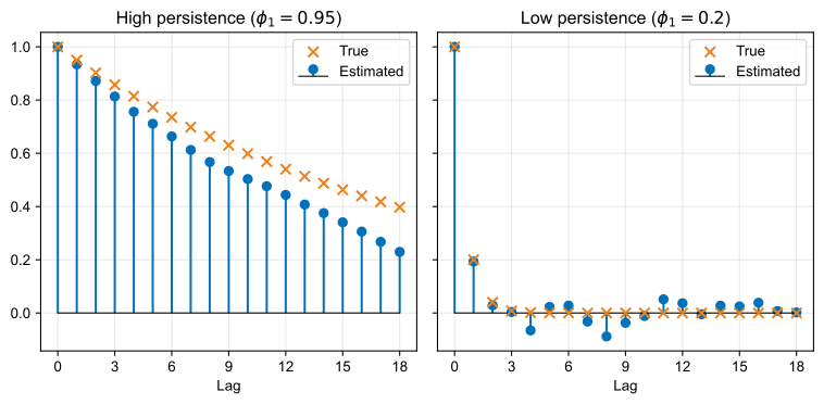
• A similar argument establishes that, in general, \(\gamma_h = \phi_1 \gamma_{h-1} \implies \gamma_h = \phi_1^h \Var(y_t)\)

How is this different from the MA(1) case?

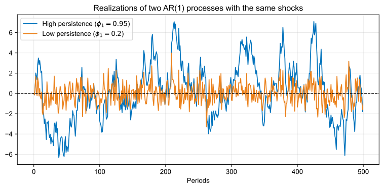
Two AR(1) Processes, Same Shocks

Estimated vs. True Autocorrelations

Unit Roots: A First Look

What Happens When \(\phi_1 = 1\)?

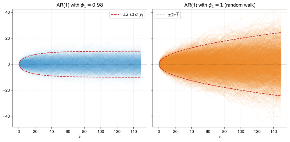
The Random Walk

• With \(\phi_1 = 1\) and \(\mu = 0\): \(y_t = y_{t-1} + \varepsilon_t = y_0 + \sum_{s=1}^{t} \varepsilon_s\)
• \(\Var(y_t \mid y_0) = t\sigma^2\) grows without bound: not stationary
• The root of \(f(x) = 1 - x\) is \(x = 1\): right on the unit circle
• Shocks never die out: \(\partial y_t / \partial \varepsilon_s = 1\) for every \(s \leq t\)
• Much more on unit roots in Lecture 8

Back to the General AR(p)

The General AR(p) Case

• Consider the general AR(p) process \(y_t = \mu + \sum_{i=1}^{p} \phi_i y_{t-i} + \varepsilon_t\)
• Let’s assume it is stationary
• The mean is easy, it follows the same tricks as before: \(\E[y_t] = \frac{\mu}{1 - \phi_1 - \phi_2 - \dots - \phi_p}\)

The variance is more involved: \[ \begin{aligned} \gamma_0 &= \Cov(y_t, y_t) \\ &= \Cov(\mu + \phi_1 y_{t-1} + \dots + \phi_p y_{t-p} + \varepsilon_t, y_t) \\ &= \phi_1 \gamma_1 + \phi_2 \gamma_2 + \dots + \phi_p \gamma_p + \sigma^2 \end{aligned} \]

In general, recalling that \(\gamma_h = \gamma_{-h}\), we get the Yule–Walker equations: \[ \gamma_h = \phi_1 \gamma_{h-1} + \phi_2 \gamma_{h-2} + \dots + \phi_p \gamma_{h-p}, \qquad h=1,2,3,\dots \]

• This generates a system of equations that can be solved recursively (a computer will do it)
• Exercise: derive the Yule–Walker equations

 

Questions?

 

The End

References

• Chapter 2 of Time Series Analysis, by James Hamilton (1994), for the lag operator
• Chapter 3 of Time Series Analysis, by James Hamilton (1994), for AR and MA models
• Chapter 14 of Econometrics, by Bruce Hansen (2022)
• Chapter 17 of Functional Analysis, by Peter Lax (2002), for the Neumann series