Lecture 3: Building Blocks for Time Series

Raul Riva

FGV, Brazilian School of Economics and Finance (FGV EPGE)

October 2026

Econometrics I (Part I)

Introduction

Types of Data

Common data structures in Economics:

Cross-sectional data: many units, one time period
- Grades of several students in one exam, GDP growth of several countries in a given year
Time series data: one unit, many time periods
- Inflation over time in one country, rainfall in a given area, the price of a stock
Panel data: many units, many time periods for the same units
- GDP growth of several countries over several years, prices of several products over time
Text, spatial data, images, etc.

Where We Are

So far: mostly cross-sectional methods (everything about \(Y_i\))
Next step: time series methods (everything about \(Y_t\))
Then: panel data methods (everything about \(Y_{i,t}\)), the most common type today

Next weeks: the challenges of time series data
This lecture: how time series differ from cross-sections, plus key definitions
Main reference: Time Series Analysis, by James Hamilton
Hansen’s book is a nice but short introduction

What Is a Time Series?

A time series: observations on one or more variables at equally spaced times
Example: annual population of a country
Unlike cross-sectional data, time series data is ordered
Here, time is discrete: days, months, years…
Continuous time (e.g., high-frequency finance) is a more advanced topic

Why Should You Care?

Policy evaluation: every policy takes place over time
- What’s the impact of a reform? Before vs after? Long-lasting effects? Fast die-outs?
- A very important building block for panel data methods
Forecasting: what could the future look like?
- What will inflation be next month? How many students will enroll next semester?
- How much inventory should a firm hold? Where is deforestation heading?
Nowcasting: high(er)-frequency monitoring of low-frequency variables
- What is the current state of the economy? How many people are unemployed right now?

It has very elegant math behind it!

The Role of Dependence

In cross-sectional data, we typically assume that observations are i.i.d.
If we relabel observations, we have no problems

In time series, independence is a rare exception
Their distribution might also change over time
If we relabel observations, we change the meaning of the data

Examples:

If inflation is high this month, it will likely be high next month
If a student is doing well on every exam, they will likely do well on the next one
Key difference from cross-sections: the future may depend on the past

Building Blocks

Random Variables

Formally, a time series is a stochastic process. First, what is a random variable?

Definition (Random Variable)

Given a probability space \((\Omega,\mathcal{F},\Pr)\), a random variable is a real function \(Y:\Omega\rightarrow\R\) such that \(\{\omega\in\Omega : Y(\omega)\leq c\}\in\mathcal{F}\) for all \(c\in \R\).

\(\Omega\) is a sample space. Example: the numbers on a die (1, 2, 3, 4, 5, 6)
\(\mathcal{F}\) is a collection of events. Example: even numbers
\(\Pr: \mathcal{F} \to [0,1]\) is a probability measure. Example: probability of rolling an even number

Think about an i.i.d. sample as different realizations of \(\omega\): \(Y_1 = Y(\omega_1), Y_2 = Y(\omega_2), \dots\)

Stochastic Processes

Definition (Stochastic Process, a Bit Informal)

A stochastic process is an ordered family of random variables \(\{Y_t, t \in \mathcal{T}\}\) defined on a probability space \((\Omega, \mathcal{F}, \Pr)\), where \(\mathcal{T}\) is an ordered set. For a fixed \(\omega \in \Omega\), the path \(\{Y_t(\omega), t \in \mathcal{T}\}\) is one realization of the process.

Loosely speaking:

A random variable is a way to model an uncertain number
A stochastic process is a way to model an uncertain path
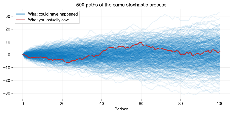
In reality, we observe one, and only one, realization of the stochastic process
Think about the history of the world: it is a single realization from \(\Omega\)
YOLO: you only live once!

YOLO

The Challenge Ahead

You observe only the red path, but the blue ones were equally likely
The challenge: you see one path but want to learn about the whole process

Example: inflation in Brazil in 1989

We know it was super high
But we have only one reading of inflation for 1989
When can one observation tell us about Brazil’s “inflation process”?

We need a lot of structure! Without it, we are lost!

Questions?

Stationarity and Ergodicity

Weak Stationarity

Definition (Weak Stationarity)

A stochastic process \(\{Y_t\}\) is weakly stationary (or second-order stationary, or covariance stationary) if, and only if, its first two unconditional population moments exist and are constant over time: \[ \begin{aligned} &\E[Y_t]=\mu, \quad |\mu|<\infty, \quad \forall\, t\in\mathcal{T}\\ &\E[(Y_t-\mu)(Y_{t-h}-\mu)]=\gamma_h, \quad |\gamma_h|<\infty, \quad \forall\, t\in\mathcal{T}, \quad h=0,\pm 1,\pm 2, \ldots \end{aligned} \]

True or false?

\(\gamma_0 = \Var(Y_t)\)
\(\gamma_h > \gamma_{-h}\) for \(h \neq 0\)
An i.i.d. process with finite variance is weakly stationary

What Process Has a Higher \(\gamma_1\)?

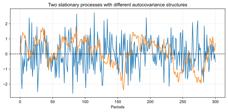
Dial the Persistence

\(Y_t = \rho\, Y_{t-1} + \sqrt{1-\rho^2}\,\varepsilon_t\) with \(\varepsilon_t \iid N(0,1)\). The shocks stay fixed: only \(\rho\) changes

viewof rho = Inputs.range([-0.95, 0.99], {value: 0.5, step: 0.01, label: "Persistence ρ"})

shocks = {
  const draw = d3.randomNormal.source(d3.randomLcg(2141))(0, 1)
  return Float64Array.from({length: 1000}, draw)
}

// Y_0 comes from the stationary law N(0, 1), so the variance is 1 for every rho
persistPath = {
  const y = new Float64Array(shocks.length)
  const s = Math.sqrt(1 - rho * rho)
  y[0] = shocks[0]
  for (let t = 1; t < y.length; t++) y[t] = rho * y[t - 1] + s * shocks[t]
  return Array.from(y, (v, t) => ({t, y: v}))
}

Plot.plot({
  width: 1200, height: 450, marginLeft: 50, marginBottom: 45,
  style: {fontSize: "19px", fontFamily: "Arial, Arimo, sans-serif"},
  x: {label: "Periods", labelAnchor: "center", labelArrow: "none"},
  y: {label: null, domain: [-4, 4], ticks: 5},
  grid: true,
  marks: [
    Plot.ruleY([0], {stroke: "black", strokeDasharray: "5,4"}),
    Plot.line(persistPath, {x: "t", y: "y", stroke: "#0072BC", strokeWidth: 1.3, clip: true})
  ]
})

Strong (or Strict) Stationarity

Definition (Strong Stationarity)

A stochastic process \(\{Y_t\}\) is strongly stationary (or strictly stationary) if, and only if, its joint distributions are invariant to time shifts: for every \(n\), every \(t_1, \dots, t_n\) and every \(\tau\), \[ F_{t_1,\ldots,t_n}(y_1,\ldots,y_n)=F_{t_1+\tau,\ldots,t_n+\tau}(y_1,\ldots,y_n) \quad \forall\, (y_1, \ldots, y_n) \] where \(F_{t_1,\ldots,t_n}\) is the joint CDF of \((Y_{t_1},\ldots,Y_{t_n})\).

True or false?

If a process is weakly stationary, it is also strongly stationary
If a process is strongly stationary, it is also weakly stationary
An i.i.d. process with finite variance is strongly stationary

Ergodicity: Motivation

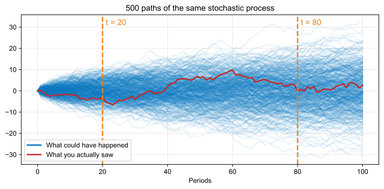
Let’s call the mysterious process from the YOLO simulation \(m_t\)
Denote by \(m_t^{(i)}\) the realization of \(m\) at time \(t\) for the \(i\)-th path
The paths are independent (because I chose so!)

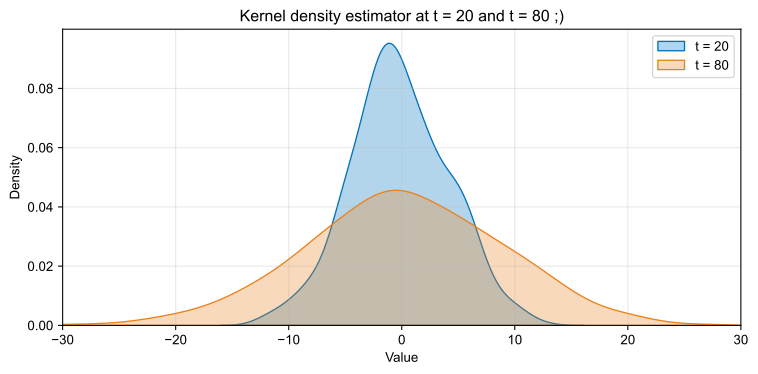
Goal: estimate two (possibly different) quantities, \(\E[m_{20}]\) and \(\E[m_{80}]\)
How can I do that?

Ergodicity: Motivation

Proposal 1: estimate \(\E[m_{20}]\) by averaging the values at \(t=20\) across all paths

Formally: \(\hat{m}_{20} = \frac{1}{n} \sum_{i=1}^{n} m_{20}^{(i)}\), where \(n\) is the number of paths. Same for \(t=80\)
Would this yield a consistent estimator?

What’s the main problem with this approach?

Proposal 2: I do not have access to the whole process, so I use the one path I have

Estimate \(\E[m_{20}]\) by averaging across all time periods in the path: \(\widetilde{m}_{20} = \frac{1}{T} \sum_{t=1}^{T} m_{t}^{(1)}\)
Would I need stationarity for this to yield a consistent estimator?
Intuitively, would that be enough?

Example: One Path, Wrong Answer

A coin is flipped once: \(Z = +2\) (“up”) or \(Z = -2\) (“down”), each with probability \(1/2\)
Then \(Y_t = Z + \varepsilon_t\), \(\varepsilon_t \iid N(0,1)\) independent of \(Z\): stationary, with \(\E[Y_t] = 0\)

viewof coin = Inputs.form({
  play: Inputs.button("Play", {value: 0, reduce: v => v + 1}),
  flip: Inputs.button("Flip a new coin", {value: 0, reduce: v => v + 1})
}, {template: ({play, flip}) => {
  for (const b of [play, flip]) { b.style.width = "auto"; b.style.margin = "0"; b.querySelector("label")?.remove() }
  return html`<div style="display: flex; justify-content: center; align-items: center; column-gap: 30px; width: 100%; max-width: none">${play}${flip}</div>`
}})

coinT = 500

// One coin flip per click of "Flip a new coin", then T shocks around Z.
// The click count is hashed into the seed: nearby LCG seeds give near-identical first draws
coinSeed = k => {
  let x = Math.imul(k ^ (k >>> 16), 0x85ebca6b)
  x = Math.imul(x ^ (x >>> 13), 0xc2b2ae35)
  return ((x ^ (x >>> 16)) >>> 0) / 4294967296
}

coinPath = {
  const rng = d3.randomLcg(coinSeed(2227 + coin.flip))
  const draw = d3.randomNormal.source(rng)(0, 1)
  const Z = rng() < 0.5 ? 2 : -2
  let sum = 0
  const rows = Array.from({length: coinT}, (_, i) => {
    const y = Z + draw()
    sum += y
    return {t: i + 1, y, avg: sum / (i + 1)}
  })
  return {Z, rows}
}

// Before any click, show the whole path (also what the print view shows); a click animates it.
// Progress follows the clock (6 s in total), so slow frames skip ahead instead of dragging
coinNow = {
  if (coin.play + coin.flip === 0) { yield coinT; return }
  const start = performance.now()
  while (true) {
    const t = Math.min(coinT, Math.max(1, Math.round((performance.now() - start) / 6000 * coinT)))
    yield t
    if (t === coinT) return
    await Promises.delay(16)
  }
}

coinShown = coinPath.rows.slice(0, coinNow)

html`<div style="text-align: center; font-size: 24px; margin-top: 10px">
  <span style="color: #0072BC; font-weight: bold">the path you see</span> &nbsp;·&nbsp;
  <span style="color: #C62828; font-weight: bold">its time average</span> &nbsp;·&nbsp;
  <span style="color: #EB811B; font-weight: bold">Z = ±2</span> &nbsp;·&nbsp;
  dashed: E[<i>Y<sub>t</sub></i>] = 0
</div>`

Plot.plot({
  width: 1200, height: 420, marginLeft: 50, marginBottom: 45,
  style: {fontSize: "19px", fontFamily: "Arial, Arimo, sans-serif"},
  x: {domain: [1, coinT], label: "Periods", labelAnchor: "center", labelArrow: "none"},
  y: {domain: [-5.5, 5.5], label: null, ticks: [-4, -2, 0, 2, 4]},
  grid: true,
  marks: [
    Plot.ruleY([-2, 2], {stroke: "#EB811B", strokeDasharray: "3,5", strokeWidth: 2}),
    Plot.ruleY([0], {stroke: "black", strokeDasharray: "7,5", strokeWidth: 1.5}),
    Plot.line(coinShown, {x: "t", y: "y", stroke: "#0072BC", strokeOpacity: 0.45, strokeWidth: 1.2}),
    Plot.line(coinShown, {x: "t", y: "avg", stroke: "#C62828", strokeWidth: 3}),
    Plot.text([`coin: ${coinPath.Z > 0 ? "up" : "down"} · time average after ${coinShown.length} periods: ${coinShown.at(-1).avg.toFixed(2)}`],
      {frameAnchor: "top-right", dx: -10, dy: 10, fill: "#C62828", fontWeight: "bold", fontSize: 20, stroke: "white", strokeWidth: 6})
  ]
})

Ergodicity: Definition

Ergodicity is a property that some stochastic processes have
Intuitive definition (don’t quote me on this):

Definition (Ergodicity, Intuitive)

A stochastic process \(\{Y_t\}\) is ergodic if its realized paths are “rich enough” with probability 1. By “rich enough”, we mean that, with probability 1, it will neither get stuck in a subset of the state space nor fall into cyclic trajectories.

In other words: observe a process for long enough and you learn everything about it

Ergodicity vs Stationarity

There are ways to test whether a process is stationary. We will get there
There is no way to test for ergodicity! You have to assume it!

Important:

When a process is stationary, there are simple conditions that imply ergodicity
Under ergodicity and strict stationarity, \(\widetilde{m}_{20}\) is consistent!
This result is called the Ergodic Theorem (Theorem 14.9 in Hansen’s book)

Also important:

Stationarity does not imply ergodicity (next slide)
Exercise (problem set): analyze a process that is stationary but not ergodic

Time Averages vs. Ensemble Averages

Two stationary processes, 50 paths each:

Ergodic: \(Y_t = \varepsilon_t\), \(\varepsilon_t \iid N(0,1)\)
Not ergodic: \(Y_t = X_t^2\), \(X_t = S\,\varepsilon_t\), \(S^2 \in \{0.5, 1.5\}\) drawn once per path (50/50)

viewof Tmax = Inputs.range([10, 5000], {value: 1000, step: 1, transform: Math.log, label: "Sample size T"})

ergo = {
  const rng = d3.randomLcg(126)
  const draw = d3.randomNormal.source(rng)(0, 1)
  const T = 5000
  const grid = Array.from(new Set(d3.range(301).map(j => Math.round(Math.exp(j * Math.log(T) / 300)))))
  return d3.range(50).map(i => {
    const S2 = rng() < 0.5 ? 0.5 : 1.5
    let sum1 = 0, sum2 = 0, k = 0
    const avgs = []
    for (let t = 1; t <= T; t++) {
      const e = draw()
      sum1 += e
      sum2 += e * e
      if (t === grid[k]) { avgs.push({t, m1: sum1 / t, m2: sum2 / t}); k++ }
    }
    return {path: i, S2, avgs}
  })
}

// Left: Y = e, so its time average is that of e. Right: Y = X^2 = S^2 e^2, so its time average is S^2 times that of e^2
ergoRows = ergo.flatMap(p => p.avgs
  .filter(d => d.t <= Tmax)
  .map(d => ({path: p.path, t: d.t, m1: d.m1, m2: p.S2 * d.m2})))

avgPanel = (key, target, domain, title) => html`<div>
  <div style="text-align: center">${title}</div>
  ${Plot.plot({
    width: 590, height: 350, marginLeft: 50, marginBottom: 45,
    style: {fontSize: "18px", fontFamily: "Arial, Arimo, sans-serif"},
    x: {type: "log", domain: [1, Tmax], label: "t (log scale)", labelAnchor: "center", labelArrow: "none"},
    y: {label: null, domain, ticks: 5},
    grid: true,
    marks: [
      Plot.ruleY([target], {stroke: "black", strokeDasharray: "7,5", strokeWidth: 1.5}),
      Plot.line(ergoRows.filter(d => d.path > 0), {x: "t", y: key, z: "path", stroke: "#0072BC", strokeOpacity: 0.3, strokeWidth: 1.3, clip: true}),
      Plot.line(ergoRows.filter(d => d.path === 0), {x: "t", y: key, stroke: "#C62828", strokeWidth: 3, clip: true}),
      Plot.text([`the path you saw: ${ergoRows.filter(d => d.path === 0).at(-1)[key].toFixed(2)}`], {frameAnchor: "top-right", dx: -10, dy: 10, fill: "#C62828", fontWeight: "bold", fontSize: 20, stroke: "white", strokeWidth: 6})
    ]
  })}
</div>`

html`<div style="display: flex; gap: 20px; justify-content: center; font-size: 19px">
${avgPanel("m1", 0, [-1.5, 1.5], html`Time average of ergodic <i>Y<sub>t</sub></i> (dashed: E[<i>Y<sub>t</sub></i>] = 0)`)}
${avgPanel("m2", 1, [0, 3], html`Time average of non-ergodic <i>Y<sub>t</sub></i> (dashed: E[<i>Y<sub>t</sub></i>] = 1)`)}
</div>`

Formal Definition: Ergodicity (Time Allowing)

Trivial Invariant Events

Let \(G \subset \R^{\infty}\) and let \(\tilde{Y}_t = (\dots, Y_{t-1}, Y_t, Y_{t+1}, \dots)\) be the history of the process
An event \(A\) has the form \(A = \{\omega \in \Omega : \tilde{Y}_t \in G\}\)
The \(l\)-th time shift of \(A\) is \(A_l = \{\omega \in \Omega : \tilde{Y}_{t+l} \in G\}\)

An event \(A\) is called invariant if \(A_l = A\) for all \(l \in \mathbb{Z}\)
An event \(A\) is called trivial if \(\Pr(A) = 0\) or \(\Pr(A) = 1\)

Definition (Ergodicity)

A process \(Y_t\) is ergodic if every invariant event is trivial.

Example

Consider the event \(A = \{\sup_{t \in \mathbb{Z}} Y_t \leq 0\}\)
In words: the process never takes a positive value

For any \(l\), \(A_l = \{\sup_{t \in \mathbb{Z}} Y_{t+l} \leq 0\}\)
Is this event invariant?

Suppose \(Y_t = Z\) for all \(t \in \mathbb{Z}\), where \(Z \sim U[-1, 1]\)
This means that the process is constant after \(Z\) is drawn
What’s \(\Pr(A)\) here?

Is this process ergodic?

One Useful Characterization of Ergodicity

Theorem (Ergodicity, Characterization)

A strictly stationary series \(Y_t \in \R^{m}\) is ergodic if, and only if, for all events \(A\) and \(B\) \[ \lim_{n \rightarrow \infty} \frac{1}{n} \sum_{l=1}^{n} \Pr(A_l \cap B) = \Pr(A) \cdot \Pr(B) \]

Intuition: as we go back in time, on average, events become nearly independent

Two Useful Theorems

Stationarity + Ergodicity = LLN

Goal: estimate the means and second moments of a process
Stationarity + ergodicity is the “right set of assumptions” to do that

Ergodic Theorem (Hayashi, 2000, pp. 101–102)

If \(Y_t\) is strictly stationary and ergodic with \(\E|Y_t| < \infty\), then \[ \bar{Y}_T = \frac{1}{T} \sum_{t=1}^{T} Y_t \xrightarrow{a.s.} \E[Y_t] \quad \text{as} \quad T \rightarrow \infty \] If, also, \(\E[Y_t^2] < \infty\), then \[ \hat{\gamma}_h = \frac{1}{T} \sum_{t=1}^{T-h} (Y_t - \bar{Y}_T)(Y_{t+h} - \bar{Y}_T) \xrightarrow{a.s.} \gamma_h \quad \text{as} \quad T \rightarrow \infty \]

What to Do in Practice?

Ergodicity cannot be tested. For estimation alone, there is an easier way out:

Theorem (Brockwell and Davis, 1991, Theorem 7.1.1)

If \(Y_t\) is weakly stationary and \(\sum_{h=0}^{\infty} |\gamma_h| < \infty\), then \[ \bar{Y}_T = \frac{1}{T} \sum_{t=1}^{T} Y_t \xrightarrow{L_2} \E[Y_t] \quad \text{as} \quad T \rightarrow \infty \]

For \(\hat{\gamma}_h \xrightarrow{p} \gamma_h\) we also need fourth moments (Brockwell and Davis, 1991, Prop. 7.3.4)
Recall: \(L_2\) implies \(\xrightarrow{p}\), but neither \(L_2\) nor a.s. convergence implies the other

Questions?

White Noise and Martingale Difference Sequences

White Noise

In the cross-section, it’s common to write \(y_i = \alpha + \beta x_i + u_i\) with \(u_i\) i.i.d.
We need weaker “error terms”: white noise and martingale difference sequences

Definition (White Noise Process)

A sequence of random variables \((\varepsilon_t)_{t \in \mathbb{Z}}\) is a white noise process if:

\(\E[\varepsilon_t] = 0\) for all \(t\)
\(\Var(\varepsilon_t) = \sigma^2 < \infty\) for all \(t\)
\(\Cov(\varepsilon_t, \varepsilon_s) = 0\) for all \(t \neq s\)

In words: uncorrelated random variables with mean zero and constant variance.

Any i.i.d. sequence with mean zero and finite variance is white noise.

Information Sets

Conditioning on past information is common in economic models and in Econometrics
The right objects are \(\sigma\)-fields and filtrations, but we skip the measure theory
Intuitively: the \(\sigma\)-field generated by \((Y_t, Y_{t-1}, \dots)\) collects the possible histories up to \(t\)
We write \(\mathcal{F}_t = \sigma(Y_t, Y_{t-1}, Y_{t-2}, \dots)\): all information available up to time \(t\)
Elsewhere in Economics, \(\sigma\)-fields are called information sets
Example: \(\E[Y_t | \mathcal{F}_{t-1}]\) is the best guess for \(Y_t\) using only this process up to \(t-1\)

Martingale Difference Sequences

Definition (Martingale Difference Sequence)

A sequence of random variables \((\varepsilon_t)_{t \in \mathbb{Z}}\) is a martingale difference sequence (MDS) with respect to the filtration \(\{\mathcal{F}_t\}\) if:

\(\varepsilon_t\) is adapted to \(\mathcal{F}_t\)
\(\E|\varepsilon_t| < \infty\) for all \(t\)
\(\E[\varepsilon_t | \mathcal{F}_{t-1}] = 0\) almost surely for all \(t\)

True or false?

Every MDS has (unconditional) mean zero
\(\Cov(\varepsilon_t, \varepsilon_{t+h}) = 0\) for all \(h \neq 0\)
\(\E[\varepsilon_{t+h} | \mathcal{F}_{t}] = 0\) for all \(h > 0\)
\(\E[\varepsilon_{t-h} | \mathcal{F}_{t}] = 0\) for all \(h > 0\)

Example

Let \(u_t\) be an i.i.d. sequence with mean zero and variance \(\sigma^2 < \infty\)
Define \(v_t = u_t \cdot u_{t-1}\)
- Is this process i.i.d.? Is it an MDS with respect to its natural filtration? Is it white noise?

Now define \(m_t = u_t + u_{t-1}\cdot u_{t-2}\)
- Is this process i.i.d.? Is it an MDS with respect to its natural filtration? Is it white noise?

The End

References

Section 2.2 of Econometrics, by Fumio Hayashi (2000)
Chapter 7 of Time Series: Theory and Methods, by Peter Brockwell and Richard Davis (1991, 2nd ed.)
Chapters 3 and 4 of Time Series Analysis, by James Hamilton. MDS are covered in Chapter 7
Chapter 14 of Econometrics, by Bruce Hansen