viewof gc = Inputs.form({
  n: Inputs.range([5, 10000], {value: 10, step: 1, transform: Math.log, label: "Sample size n"}),
  seed: Inputs.button("Draw new samples", {value: 1, reduce: v => v + 1})
}, {template: ({n, seed}) => {
  n.style.setProperty("--input-width", "420px")
  n.style.maxWidth = "none"
  return html`<div style="display: flex; justify-content: center; align-items: center; column-gap: 30px">${n}${seed}</div>`
}})Lecture 2: Bootstrap 101
Raul Riva
FGV, Brazilian School of Economics and Finance (FGV EPGE)
October 2026
Econometrics I (Part I)
Motivation
The Margin of Error You See on TV
- An online poll asks \(n\) voters whether they will vote for candidate A
- Online polls are self-selected, but let’s pretend respondents are iid today ;)
- \(X_i = 1\) if respondent \(i\) picks A, so \(p = P\{X_i = 1\}\) and \(\hat p = \bar X_n\)
- The CLT and Slutsky’s theorem give \[ \frac{\sqrt n\,(\hat p - p)}{\sqrt{\hat p(1-\hat p)}} \xrightarrow{d} N(0,1) \quad\implies\quad \hat p \pm 1.96\sqrt{\frac{\hat p(1-\hat p)}{n}} \]
- In our simulated poll, \(n = 2{,}000\) and \(\hat p =\) 37.8%, so the interval is \(\hat p \pm\) 2.1 p.p.
- Two ingredients: a known limit, and a nuisance parameter we can estimate
Now the Whole TV Graphic
Each respondent also declares a state. Here are 18 95% intervals from the same poll:
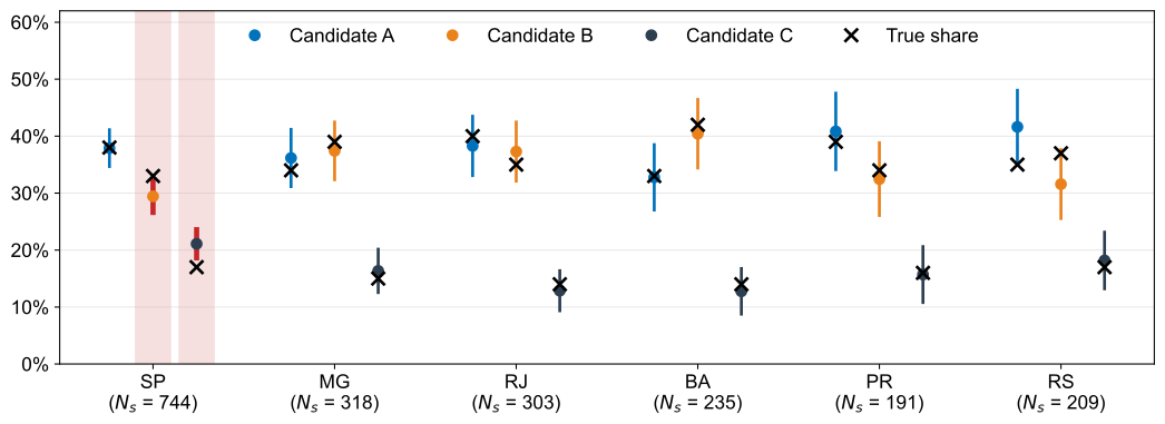
- Each interval is right 95% of the time. What’s the chance that all 18 are right?
- Simulating many polls from the truth: only about 42%. The red ones missed
A Joint Confidence Set
- \(p_{s,k}\): share of candidate \(k \in \{A, B, C\}\) among voters in state \(s\)
- \(N_s\): number of respondents from state \(s\), and \(\widehat{se}_{s,k} = \sqrt{\hat p_{s,k}(1-\hat p_{s,k})/N_s}\)
- We want one statement about all 18 shares at once:
\[ P\left\{ p_{s,k} \in \left[\hat p_{s,k} - c\cdot \widehat{se}_{s,k},\ \hat p_{s,k} + c\cdot \widehat{se}_{s,k}\right] \text{ for every } s, k \right\} = 1 - \alpha \]
- Same form as on TV: only the multiplier \(c\) changes
- \(c = 1.96\) is too small. How large must \(c\) be?
From 18 Intervals to One Statistic
Let \(t_{s,k} \equiv (\hat p_{s,k} - p_{s,k})/\widehat{se}_{s,k}\), the usual t-statistic. Then \[ \text{all 18 intervals cover} \iff |t_{s,k}| \le c \ \text{ for every } s,k \iff \underbrace{\max_{s,k}\, |t_{s,k}|}_{\equiv\, R_n} \le c \]
- So \(c\) is the \(1-\alpha\) quantile of \(R_n\): the whole problem boils down to one number
- Easy, right?
- . . . but what is the distribution of \(R_n\)?
What Is the Distribution of \(R_n\)?
- \((t_{s,k})_{s,k} \xrightarrow{d} Z \sim N(0, \Sigma)\): CLT, delta method and Slutsky
- \(R_n \xrightarrow{d} \max_{s,k}|Z_{s,k}|\): continuous mapping theorem, since the max is continuous
- Across states, the \(Z\)’s are independent. Within a state, candidates compete for voters: \[ \Corr(Z_{s,j}, Z_{s,k}) = -\sqrt{\frac{p_{s,j}\, p_{s,k}}{(1-p_{s,j})(1-p_{s,k})}}, \qquad j \neq k \]
- The maximum of 18 correlated normals has no closed-form quantile
- And that quantile depends on the unknown shares \(p_{s,k}\)
What we really want
The distribution of \(R_n\) at our sample size, without having to derive its limit.
The Idea in Words
- If we knew how everyone votes, we would simulate many polls and compute \(R_n\) in each
- The \(95\%\) quantile of the simulated \(R_n\)’s would be our \(c\). But we don’t know that…
- What we do have: our 2,000 respondents, a miniature of the electorate
- Bootstrap: pretend our sample is the electorate, and simulate polls from it
- Simulating a poll from the sample = drawing 2,000 respondents with replacement
- Efron (1979): you pull yourself up by your bootstraps
- Dark magic? Do they teach this at Hogwarts? No: it’s just the plug-in principle!
- Today: the non-parametric bootstrap with iid data
Roots and Pivots
Setup
- Data: \(X^n = (X_1, \dots, X_n)\), iid with unknown distribution \(P \in \mathcal{P}\)
- The model \(\mathcal{P}\) can be parametric, semiparametric or nonparametric
- Parameter of interest: \(\theta(P) \in \Theta \equiv \{\theta(P) : P \in \mathcal{P}\}\)
- Goal: a random set \(C_n = C_n(X^n)\) such that \(P\{\theta(P) \in C_n\} \approx 1-\alpha\)
Definition (Root)
A root is any real-valued function \(R_n(X^n, \theta(P))\) of the data and of the parameter.
- The name is due to Beran (1984)
- Examples: \(\sqrt n\,(\hat\theta_n - \theta(P))\) and \(\sqrt n\,(\hat\theta_n - \theta(P))/\hat\sigma_n\)
- In the poll: \(\theta(P)\) stacks the 18 shares, and \(R_n = \max_{s,k}|t_{s,k}|\)
The Object of Interest
Definition (Sampling Distribution of the Root)
\[ \begin{aligned} J_n(x, P) &\equiv P\left\{R_n(X^n, \theta(P)) \le x\right\}\\ J_n^{-1}(1-\alpha, P) &\equiv \inf\left\{x : J_n(x, P) \ge 1-\alpha\right\} \end{aligned} \]
- \(J_n\) depends on the sample size \(n\) and on the unknown \(P\)
- The infimum handles discrete distributions, where quantiles may not be unique
- If we knew \(J_n(\cdot, P)\), we could invert the root: \[ C_n = \left\{\theta \in \Theta : J_n^{-1}(\tfrac{\alpha}{2}, P) \le R_n(X^n, \theta) \le J_n^{-1}(1 - \tfrac{\alpha}{2}, P)\right\} \]
- By construction, \(P\{\theta(P) \in C_n\} \ge 1 - \alpha\), with equality if \(J_n\) is continuous
From \(J_n\) to an Interval
- With \(R_n = \sqrt n\,(\hat\theta_n - \theta)\), the two inequalities that define \(C_n\) read \[ J_n^{-1}(\tfrac{\alpha}{2}, P) \le \sqrt n\,(\hat\theta_n - \theta) \le J_n^{-1}(1 - \tfrac{\alpha}{2}, P) \]
- Solve for \(\theta\): \[ \hat\theta_n - \frac{J_n^{-1}(1-\frac{\alpha}{2}, P)}{\sqrt n} \le \theta \le \hat\theta_n - \frac{J_n^{-1}(\frac{\alpha}{2}, P)}{\sqrt n} \]
- If \(J_n\) is symmetric around zero, this is just \(\hat\theta_n \pm J_n^{-1}(1-\frac{\alpha}{2}, P)/\sqrt n\)
The goal of this lecture
We want a confidence set for \(\theta(P)\). For that, all we need is \(J_n(\cdot, P)\).
Pivots
Definition (Pivot)
The root \(R_n(X^n, \theta(P))\) is a pivot if \(J_n(x, P) = J_n(x)\) for all \(x\) and all \(P \in \mathcal{P}\).
Examples:
- \(X_i \iid N(\theta, 1)\): \(\ \sqrt n\,(\bar X_n - \theta) \sim N(0,1)\), whatever \(\theta\) is
- \(X_i \iid N(\mu, \sigma^2)\): \(\ \sqrt n\,(\bar X_n - \mu)/S_n \sim t_{n-1}\), whatever \(\mu\) and \(\sigma\) are
Not pivots:
- \(X_i \iid N(\mu, \sigma^2)\): \(\ \sqrt n\,(\bar X_n - \mu) \sim N(0, \sigma^2)\), which depends on \(\sigma\)
- \(X_i \iid P\), any \(P\) with finite variance: the law of \(\sqrt n\,(\bar X_n - \mu)/S_n\) depends on \(P\)
Why Pivots Are Great
- Coverage is exact: \(P\{\theta(P) \in C_n\} = 1-\alpha\) for every \(n\) and every \(P \in \mathcal{P}\)
- No asymptotics at all: \(n = 15\) is as good as \(n = 15{,}000\)
- Only one distribution to learn: look it up once in a table (think \(t_{n-1}\))
- Bootstrap preview: we will replace \(P\) by an estimate \(\hat P_n\)
- The less \(J_n(\cdot, P)\) depends on \(P\), the less that replacement hurts
- Moral, and we will come back to it: bootstrap a pivot whenever you can
- Location-scale model: \(X_i = \theta + \sigma\varepsilon_i\), with \(\varepsilon_i \iid F\) and \(F\) known, but \((\theta, \sigma)\) unknown
- Exercise: show that \((\bar X_n - \theta)/S_n\) is a pivot (L&R Problem 18.1)
Not Pivots
Being a pivot is a property of the root and of the model \(\mathcal{P}\):
- Two normal samples with \(\sigma_X \neq \sigma_Y\): the law of Welch’s \(T\) depends on \(\sigma_X/\sigma_Y\) \[ T = \frac{(\bar X - \bar Y) - (\mu_X - \mu_Y)}{\sqrt{S_X^2/n_X + S_Y^2/n_Y}} \]
- Proportions: the law of \(\sqrt n\,(\hat p - p)/\sqrt{\hat p(1-\hat p)}\) is discrete and depends on \(p\)
- That’s the root behind the TV margin of error, so its coverage swings with \(p\) and \(n\)
- See Brown, Cai and DasGupta (2001) for how erratic it gets
Asymptotic Pivots
Definition (Asymptotic Pivot)
The root is an asymptotic pivot if, for every \(P \in \mathcal{P}\), \(J_n(\cdot, P)\) converges weakly to the same limit \(J\), which does not depend on \(P\).
- The t-statistic: if \(0 < \sigma^2(P) < \infty\), then \(\sqrt n\,(\bar X_n - \theta(P))/S_n \xrightarrow{d} N(0,1)\)
- That’s the TV margin of error: it holds for every \(P\) with finite variance
- Parametric models where \(\hat{\theta}_n\) is the MLE: \(n(\hat\theta_n - \theta)'I(\hat\theta_n)(\hat\theta_n - \theta) \xrightarrow{d} \chi^2_k\) (Wald)
- Recipe: build \(C_n\) with the quantiles of \(J\) instead of those of \(J_n\)
- The price: coverage is only right in the limit, \(\lim_{n} P\{\theta(P) \in C_n\} = 1-\alpha\)
When the Limit Depends on \(P\)
- The typical case: \(J_n(\cdot, P) \to J(\cdot, P)\), and the limit depends on \(P\)
- Example: \(\sqrt n\,(\bar X_n - \theta(P)) \xrightarrow{d} N(0, \sigma^2(P))\), so use \(J(x, \hat P_n) = \Phi(x/\hat\sigma_n)\)
- This only works if you know \(J(\cdot, P)\) and can estimate whatever it depends on
- Median: \(\sqrt n\,(\hat m_n - m) \xrightarrow{d} N\big(0, 1/(4f(m)^2)\big)\): needs \(\hat f(m)\) (Lecture 1!)
- In the poll, \(J(\cdot, P)\) is the law of \(\max_{s,k}|Z_{s,k}|\): no closed form at all
- Even then, it’s a double approximation: \(J_n(\cdot, P) \approx J(\cdot, P) \approx J(\cdot, \hat P_n)\)
Two Ways to Approximate \(J_n(x, P)\)
\[ \begin{aligned} \textbf{Asymptotics:}&\quad J_n(x, P) \;\underset{n \to \infty}{\approx}\; J(x, P) \;\approx\; J(x, \hat P_n)\\[10pt] \textbf{Bootstrap:}&\quad J_n(x, P) \;\underset{n \to \infty}{\approx}\; J_n(x, \hat P_n) \end{aligned} \]
- Asymptotics: replace \(J_n\) by its limit \(J\), whose formula you must derive
- If \(J\) depends on \(P\) (not an asymptotic pivot), also estimate it: \(J(x, \hat P_n)\)
- Bootstrap: keep \(J_n\), and plug \(\hat P_n\) into \(J_n\) itself
- \(J\) never shows up: no limit to derive, no nuisance parameter to estimate
Read this twice (and then maybe get a tattoo!)
The bootstrap does not avoid asymptotics. What it avoids is having to know \(J\).
Questions?
The Bootstrap
The Bootstrap Estimator
- Estimate \(P\) by the empirical distribution, which puts mass \(1/n\) on each \(X_i\): \[ \hat P_n(E) \equiv \frac{1}{n}\sum_{i=1}^n I\{X_i \in E\} \]
- The bootstrap estimator of the sampling distribution is a plug-in: \(J_n(x, \hat P_n)\)
- Unusual target: \(J_n(\cdot, P)\) changes with \(n\), and we estimate it at our \(n\)
- The bootstrap confidence set replaces \(P\) by \(\hat P_n\) in the quantiles: \[ C_n^{*} = \left\{\theta \in \Theta : J_n^{-1}(\tfrac{\alpha}{2}, \hat P_n) \le R_n(X^n, \theta) \le J_n^{-1}(1-\tfrac{\alpha}{2}, \hat P_n)\right\} \]
- Two questions: is \(J_n(\cdot, \hat P_n)\) close to \(J_n(\cdot, P)\)? And how do we compute it?
Why Should \(\hat P_n\) Be Close to \(P\)?
- With real-valued data, \(\hat F_n(t) \equiv \hat P_n\big((-\infty, t]\big)\) is the empirical CDF
- Fixed \(t\): \(\hat F_n(t) \to F(t)\) a.s. by the SLLN, since \(\E\left[I\{X_i \le t\}\right] = F(t)\)
- We can do much better: the convergence is uniform in \(t\)
Theorem (Glivenko–Cantelli)
If \(X_1, \dots, X_n\) are iid real-valued random variables with CDF \(F\), then \[ \sup_{t \in \R} \left|\hat F_n(t) - F(t)\right| \to 0 \quad \text{almost surely} \]
- And fast: \(P\left\{\sup_t |\hat F_n(t) - F(t)| > d\right\} \le 2e^{-2nd^2}\) for every \(n\) (DKW inequality)
Glivenko–Cantelli Works, Baby!
\(X_i \iid U[0,1]\), so \(F(t) = t\) (dashed). Raising \(n\) adds draws to the same samples
gcMaxN = 10000
gcCloud = 100
gcCache = new Map()
gcStreams = {
  if (!gcCache.has(gc.seed)) {
    const unif = d3.randomLcg(gc.seed)
    gcCache.clear()
    gcCache.set(gc.seed, d3.range(gcCloud + 2).map(() => Float64Array.from({length: gcMaxN}, unif)))
  }
  return gcCache.get(gc.seed)
}

// sup_t |F_n(t) - t| from a sorted sample (the Kolmogorov-Smirnov distance)
function supGap(xs) {
  const n = xs.length
  let d = 0
  for (let i = 0; i < n; i++) d = Math.max(d, (i + 1) / n - xs[i], xs[i] - i / n)
  return d
}

// ECDF as points for a step-after line: exact jumps for small n, a fine grid for large n
function ecdfPoints(xs) {
  const n = xs.length
  if (n <= 400) return [[0, 0], ...Array.from(xs, (x, i) => [x, (i + 1) / n]), [1, 1]]
  const pts = []
  for (let g = 0, j = 0; g <= 500; g++) {
    while (j < n && xs[j] <= g / 500) j++
    pts.push([g / 500, j / n])
  }
  return pts
}

gcSorted = gcStreams.map(s => s.slice(0, gc.n).sort())
gcGaps = gcSorted.map(supGap)
dkw = Math.sqrt(Math.log(2 / 0.05) / (2 * gc.n))
gcInside = gcGaps.slice(2).filter(d => d <= dkw).length

gcStyle = ({
  width: 560, height: 450, marginLeft: 45, marginRight: 15, marginBottom: 45,
  style: {fontSize: "18px", fontFamily: "Arial, Arimo, sans-serif"},
  x: {label: "t", domain: [0, 1], ticks: 5, labelAnchor: "center", labelArrow: "none"},
  y: {label: null, domain: [0, 1], ticks: 5},
  grid: true
})
gcLabel = (text, dy, fill) => Plot.text([text], {frameAnchor: "top-left", dx: 10, dy, fill, fontWeight: "bold", fontSize: 19, stroke: "white", strokeWidth: 6})
gcTitle = text => html`<div style="text-align: center; font-weight: bold; font-size: 22px; color: #2D3E50">${text}</div>`

gcLeft = Plot.plot({...gcStyle, marks: [
  Plot.line([[0, 0], [1, 1]], {stroke: "black", strokeWidth: 1.5, strokeDasharray: "6,5"}),
  Plot.line(ecdfPoints(gcSorted[0]), {curve: "step-after", stroke: "#0072BC", strokeWidth: 2.5}),
  Plot.line(ecdfPoints(gcSorted[1]), {curve: "step-after", stroke: "#EB811B", strokeWidth: 2.5}),
  gcLabel(`Sample 1: sup gap = ${gcGaps[0].toFixed(3)}`, 8, "#0072BC"),
  gcLabel(`Sample 2: sup gap = ${gcGaps[1].toFixed(3)}`, 36, "#EB811B")
]})

gcRight = {
  const band = d3.range(0, 1.0001, 0.005).map(t => ({t, lo: Math.max(0, t - dkw), hi: Math.min(1, t + dkw)}))
  const cloud = gcSorted.slice(2).flatMap((xs, id) => ecdfPoints(xs).map(([t, y]) => ({t, y, id})))
  return Plot.plot({...gcStyle, marks: [
    Plot.areaY(band, {x: "t", y1: "lo", y2: "hi", fill: "#2D3E50", fillOpacity: 0.12}),
    Plot.line(cloud, {x: "t", y: "y", z: "id", curve: "step-after", stroke: "#0072BC", strokeOpacity: 0.25, strokeWidth: 1.2}),
    Plot.line([[0, 0], [1, 1]], {stroke: "black", strokeWidth: 1.5, strokeDasharray: "6,5"}),
    gcLabel(`DKW 95% band: ± ${dkw.toFixed(3)}`, 8, "#2D3E50"),
    gcLabel(`${gcInside} of ${gcCloud} samples inside it`, 36, "#0072BC")
  ]})
}

html`<div style="display: flex; justify-content: center; column-gap: 30px">
  <div>${gcTitle("Two samples, one path each")}${gcLeft}</div>
  <div>${gcTitle(`${gcCloud} samples`)}${gcRight}</div>
</div>`
Is That Enough?
- Glivenko–Cantelli: \(\hat P_n\) is close to \(P\)
- But we need more: \(J_n(\cdot, \hat P_n)\) close to \(J_n(\cdot, P)\)
- That requires \(J_n(\cdot, P)\) to be continuous in \(P\): close inputs, close outputs
Two ingredients, which we will make precise soon:
- \(\hat P_n \to P\) in some sense (Glivenko–Cantelli, the SLLN)
- Whenever a sequence \({P_n}\) converges to \(P\) in that sense, \(J_n(\cdot, P_n) \to J(\cdot, P)\)
- Ingredient 2 is the delicate one. We will meet a root for which it fails: the maximum!
- Notice that item 2) is a continuity property of the root, not of the estimator \(\hat P_n\)
In Practice
How Many Bootstrap Samples Are There?
- Goal: compute \(J_n(x, \hat P_n)\), the law of the root when the data come from \(\hat P_n\)
- Under \(\hat P_n\), each of the \(n\) draws picks one of \(X_1, \dots, X_n\) with probability \(1/n\)
- Exercise: how many ordered samples of size \(n\) can we draw from \(\hat P_n\)?
- \(n^n\), all equally likely: \(J_n(x, \hat P_n)\) is an average over \(n^n\) samples
- For \(n = 100\), that’s \(10^{200}\) samples. Atoms in the universe: about \(10^{80}\)
- Exact computation is hopeless for any realistic \(n\)
Computing \(J_n(x, \hat P_n)\)
- So we simulate. Conditional on the data:
Algorithm: repeat steps 1 and 2 for \(b = 1, \dots, B\)
- Draw \(n\) observations with replacement from the data: \(X^{n*}_b = (X^*_{1,b}, \dots, X^*_{n,b})\)
- Compute the root at the plug-in parameter: \(R^*_{n,b} = R_n(X^{n*}_b, \hat\theta_n)\), with \(\hat\theta_n = \theta(\hat P_n)\)
- Compute the empirical CDF of the \(B\) roots: \(L_n(x) \equiv \frac{1}{B}\sum_{b=1}^B I\{R^*_{n,b} \le x\}\)
- Use the quantiles of \(L_n\) in place of those of \(J_n(\cdot, P)\)
- Two sources of randomness are floating around here. Which ones?
Bootstrapping the Poll, Step by Step
- In general, swap the quantiles of \(J_n(\cdot, P)\) for the left and right quantiles of \(L_n\): \[ C_n^* = \left\{\theta \in \Theta : L_n^{-1}(\tfrac{\alpha}{2}) \le R_n(X^n, \theta) \le L_n^{-1}(1 - \tfrac{\alpha}{2})\right\} \]
- In the poll, \(R_n \ge 0\) and only large values are bad news: we need just \(L_n^{-1}(1-\alpha)\)
The poll, with \(B = 1{,}000\)
- Draw 2,000 respondents (state and vote) with replacement from our poll
- Recompute the 18 shares \(\hat p^*_{s,k}\) and their standard errors \(\widehat{se}^*_{s,k}\)
- Store \(R^*_{n,b} = \max_{s,k}|\hat p^*_{s,k} - \hat p_{s,k}|/\widehat{se}^*_{s,k}\), and repeat steps 1 to 3 \(B\) times
- Set \(\hat c^{\,*} = L_n^{-1}(1-\alpha)\) and report \(\hat p_{s,k} \pm \hat c^{\,*}\,\widehat{se}_{s,k}\) for all 18 shares
- Step 3 centers at \(\hat p_{s,k}\), not \(p_{s,k}\): under \(\hat P_n\), the true shares are \(\hat p_{s,k}\)
Back to the Poll
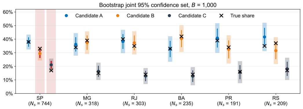
- Thin bars: \(\pm 1.96\,\widehat{se}\). Shaded bars: the joint rectangle, \(\pm \hat c^{\,*}\widehat{se}\) with \(\hat c^{\,*} =\) 3.08
- Over 500 (newly simulated) polls, each with its own \(\hat c^{\,*}\), all 18 covered: 44% with \(\pm 1.96\), 95% with \(\pm \hat c^{\,*}\)
Play With \(n\) and \(B\)
Bars: \(B\) bootstrap draws from one poll. Curve: the true \(J_n\) (100,000 polls from \(P\))
viewof demo = Inputs.form({
  n: Inputs.radio([1000, 2000, 5000, 10000, 20000], {value: 1000, label: "Poll size n", format: d => d.toLocaleString("en-US")}),
  B: Inputs.range([50, 10000], {value: 200, step: 1, transform: Math.log, label: "Bootstrap draws B"}),
  poll: Inputs.button("Draw a new poll", {value: 1, reduce: v => v + 1})
}, {template: ({n, B, poll}) => {
  n.style.setProperty("--input-width", "560px")
  n.style.maxWidth = "none"
  B.style.setProperty("--input-width", "300px")
  return html`<div style="display: flex; flex-direction: column; align-items: center">
    ${n}<div style="display: flex; align-items: center; column-gap: 30px">${B}${poll}</div>
  </div>`
}})
function rmultinom(n, pr, binom) {
const out = new Array(pr.length).fill(0)
let left = n, mass = 1
for (let j = 0; j < pr.length - 1 && left > 0; j++) {
const q = Math.min(1, Math.max(0, pr[j] / mass))
out[j] = q > 0 ? binom(left, q)() : 0
left -= out[j]
mass -= pr[j]
}
out[pr.length - 1] += left
return out
}
// max_{s,k} |t_{s,k}| for 6 states x 4 votes (the first 3 votes are candidates)
function maxT(counts, pRef) {
let m = 0
for (let s = 0; s < 6; s++) {
const N = counts[4 * s] + counts[4 * s + 1] + counts[4 * s + 2] + counts[4 * s + 3]
for (let k = 0; k < 3; k++) {
const p = counts[4 * s + k] / N
const t = Math.abs(p - pRef[3 * s + k]) / Math.sqrt(p * (1 - p) / N)
m = Math.max(m, Number.isNaN(t) ? Infinity : t)
}
}
return m
}
pollCounts = rmultinom(demo.n, poll_probs, d3.randomBinomial.source(d3.randomLcg(1000 + demo.poll)))
pollShares = d3.range(18).map(i => {
const s = Math.floor(i / 3), k = i % 3
const c = pollCounts.slice(4 * s, 4 * s + 4)
return c[k] / d3.sum(c)
})
bootR = {
const binom = d3.randomBinomial.source(d3.randomLcg(7 + 31 * demo.poll))
const freq = pollCounts.map(c => c / demo.n)
return Float64Array.from({length: demo.B}, () => maxT(rmultinom(demo.n, freq, binom), pollShares))
}
cStar = d3.quantile(bootR, 0.95)
truthN = poll_truth[String(demo.n)]
bw = poll_edges[1] - poll_edges[0]
histBoot = poll_edges.slice(0, -1).map((x0, i) => {
const x1 = poll_edges[i + 1]
const inBin = bootR.filter(r => (i === 0 ? true : r >= x0) && (i === poll_edges.length - 2 ? true : r < x1)).length
return {x0, x1, dens: inBin / (demo.B * bw)}
})
truthLine = truthN.dens.map((d, i) => ({x: (poll_edges[i] + poll_edges[i + 1]) / 2, dens: d}))
Plot.plot({
width: 1150, height: 390, marginLeft: 50, marginBottom: 45,
style: {fontSize: "20px", fontFamily: "Arial, Arimo, sans-serif"},
x: {label: "max |t|", domain: [1, 5.5], labelAnchor: "center", labelArrow: "none"},
y: {label: null, domain: [0, 1.6], ticks: 4},
grid: true,
marks: [
Plot.rectY(histBoot, {x1: "x0", x2: "x1", y: "dens", fill: "#0072BC", fillOpacity: 0.35, inset: 0.5}),
Plot.line(truthLine, {x: "x", y: "dens", stroke: "#2D3E50", strokeWidth: 3, curve: "basis"}),
Plot.ruleX([1.96], {stroke: "#EB811B", strokeWidth: 3, strokeDasharray: "7,5"}),
Plot.ruleX([poll_c_limit], {stroke: "#888888", strokeWidth: 2, strokeDasharray: "3,4"}),
Plot.ruleX([truthN.c], {stroke: "#2D3E50", strokeWidth: 3}),
Plot.ruleX([cStar], {stroke: "#0072BC", strokeWidth: 3}),
Plot.text([`bootstrap ĉ* = ${cStar.toFixed(2)}`], {frameAnchor: "top-right", dx: -10, dy: 8, fill: "#0072BC", fontWeight: "bold", fontSize: 21, stroke: "white", strokeWidth: 6}),
Plot.text([`true c = ${truthN.c.toFixed(2)}`], {frameAnchor: "top-right", dx: -10, dy: 36, fill: "#2D3E50", fontWeight: "bold", fontSize: 21, stroke: "white", strokeWidth: 6}),
Plot.text([`limit = ${poll_c_limit.toFixed(2)}`], {frameAnchor: "top-right", dx: -10, dy: 64, fill: "#888888", fontWeight: "bold", fontSize: 21, stroke: "white", strokeWidth: 6}),
Plot.text([`TV: 1.96 covers all 18 only ${Math.round(100 * truthN.cov196)}% of the time`], {frameAnchor: "top-right", dx: -10, dy: 92, fill: "#EB811B", fontWeight: "bold", fontSize: 21, stroke: "white", strokeWidth: 6})
]
})Questions?
Why It Works
Consistency: The General Recipe
Theorem (L&R 18.3.1)
Let \(\mathcal{C}_P\) be a set of sequences \(\{P_n\}\) that contains \(\{P, P, \dots\}\). Assume that, for every \(\{P_n\} \in \mathcal{C}_P\), \(J_n(\cdot, P_n)\) converges weakly to the same continuous limit \(J(\cdot, P)\). If \(\{\hat P_n\} \in \mathcal{C}_P\) with probability one, then:
\(\ \sup_x \left|J_n(x, \hat P_n) - J_n(x, P)\right| \to 0\) almost surely
\(\ J_n^{-1}(1-\alpha, \hat P_n) \to J^{-1}(1-\alpha, P)\) almost surely, if \(J(\cdot, P)\) is strictly increasing at \(J^{-1}(1-\alpha, P)\)
\(\ P\left\{R_n(X^n, \theta(P)) \le J_n^{-1}(1-\alpha, \hat P_n)\right\} \to 1-\alpha\)
- Think of \(\mathcal{C}_P\) as the sequences with \(d(P_n, P) \to 0\), for some metric \(d\)
- Part (iii): the bootstrap confidence set has asymptotically correct coverage
Proof of (i) and (ii)
- Fix a nonrandom \(\{P_n\} \in \mathcal{C}_P\). Since \(J(\cdot, P)\) is continuous, Pólya’s theorem gives \[ \sup_x |J_n(x, P_n) - J(x, P)| \to 0 \quad\text{and}\quad \sup_x |J_n(x, P) - J(x, P)| \to 0 \]
- The second one uses the constant sequence \(\{P, P, \dots\} \in \mathcal{C}_P\). By the triangle inequality: \[ \sup_x |J_n(x, P_n) - J_n(x, P)| \le \sup_x |J_n(x, P_n) - J(x, P)| + \sup_x |J(x, P) - J_n(x, P)| \to 0 \]
- Now the randomness: fix an \(\omega\) in the probability-one event where \(\{\hat P_n(\omega)\} \in \mathcal{C}_P\)
- Along that path, \(\{\hat P_n(\omega)\}\) is just a nonrandom sequence in \(\mathcal{C}_P\): apply the above \(\implies\) (i)
- For (ii): if \(F_n \Rightarrow F\), then \(F_n^{-1}(1-\alpha) \to F^{-1}(1-\alpha)\) (L&R Lemma 11.2.1)
- This needs \(F\) continuous and strictly increasing at \(F^{-1}(1-\alpha)\)
- Apply it path by path, with \(F_n = J_n(\cdot, \hat P_n(\omega))\) and \(F = J(\cdot, P)\) \(\implies\) (ii)
Proof of (iii): Two Ingredients
- Shorthand: \(R_n \equiv R_n(X^n, \theta(P))\), \(\ \hat c_n \equiv J_n^{-1}(1-\alpha, \hat P_n)\), \(\ c \equiv J^{-1}(1-\alpha, P)\)
- Goal: show \(P\{R_n \le \hat c_n\} \to 1-\alpha\)
- The root converges. Under \(P\), the CDF of \(R_n\) is \(J_n(\cdot, P)\), by definition
- \(\{P, P, \dots\} \in \mathcal{C}_P\), so the assumption gives \(J_n(\cdot, P) \Rightarrow J(\cdot, P)\), i.e., \[ R_n \xrightarrow{d} R, \qquad R \sim J(\cdot, P) \]
- The critical value converges. By (ii), \(\hat c_n \to c\) almost surely, so also in probability
- The limit \(c\) is a constant, which is what Slutsky needs
Proof of (iii): Putting Them Together
- By Slutsky, combining \(R_n \xrightarrow{d} R\) and \(\hat c_n \xrightarrow{p} c\): \[ R_n - \hat c_n \xrightarrow{d} R - c, \qquad P\{R - c \le x\} = P\{R \le x + c\} = J(x + c, P) \]
- \(J(\cdot, P)\) is continuous, so \(x = 0\) is a continuity point of the limit CDF \(J(\cdot + c, P)\): \[ P\{R_n \le \hat c_n\} = P\{R_n - \hat c_n \le 0\} \to J(c, P) \]
- Last step: \(J(c, P) = 1-\alpha\). Recall \(c = \inf\{x : J(x, P) \ge 1-\alpha\}\)
- \(J(c, P) \ge 1-\alpha\): \(J(\cdot, P)\) is right-continuous
- \(J(c, P) \le 1-\alpha\): \(J(x, P) < 1-\alpha\) for every \(x < c\), and \(J(\cdot, P)\) is continuous \[ P\{R_n \le \hat c_n\} \to J(c, P) = 1-\alpha \qquad \blacksquare \]
Reading the Theorem
- All the work is in the assumption: \(J_n(\cdot, P_n) \to J(\cdot, P)\) along every sequence in \(\mathcal{C}_P\)
- That is a form of continuity of \(J_n\) in \(P\), uniformly in \(n\): “local uniformity”
- Why sequences? \(\hat P_n\) is random, but each realized path is a nonrandom sequence
- So: first study nonrandom \(\{P_n\}\), then plug in \(\{\hat P_n\}\) path by path
- The right notion of “\(P_n \to P\)”, i.e., the set \(\mathcal{C}_P\), depends on the root
- The bigger \(\mathcal{C}_P\) can be, the easier it is to show that \(\{\hat P_n\} \in \mathcal{C}_P\)
- Recipe for a new root: (1) find \(\mathcal{C}_P\) with \(J_n(\cdot, P_n) \to J(\cdot, P)\); (2) show \(\{\hat P_n\} \in \mathcal{C}_P\)
The Nonparametric Mean
Theorem (L&R 18.3.3)
Let \(F\) have finite, nonzero variance \(\sigma^2(F)\) and mean \(\theta(F)\). Let \(J_n(\cdot, F)\) be the distribution of \(R_n = \sqrt n\,(\bar X_n - \theta(F))\) under \(F\).
Let \(\mathcal{C}_F\) be the set of sequences \(\{F_n\}\) such that \(F_n \Rightarrow F\), \(\theta(F_n) \to \theta(F)\) and \(\sigma^2(F_n) \to \sigma^2(F)\). For every \(\{F_n\} \in \mathcal{C}_F\), \(J_n(\cdot, F_n)\) converges weakly to \(N(0, \sigma^2(F))\).
If \(X_1, \dots, X_n\) are iid \(F\), then the bootstrap \(J_n(\cdot, \hat F_n)\) is consistent: (i)–(iii) of the previous theorem hold.
- Part (i) is a CLT for a triangular array: row \(n\) is iid from \(F_n\), which changes with \(n\)
- That’s exactly what resampling from \(\hat F_n\) looks like: a new distribution for each \(n\)
Proof of (i): A Triangular Array
- \(F_n\) changes with \(n\), so each \(n\) needs its own sample. Row \(n\) is \(X_{n,1}, \dots, X_{n,n}\) iid \(F_n\): \[ \begin{array}{llll} X_{1,1} & & & \sim F_1 \\ X_{2,1} & X_{2,2} & & \sim F_2 \\ X_{3,1} & X_{3,2} & X_{3,3} & \sim F_3 \\ \vdots & & & \ \ \vdots \end{array} \]
- Center at the row’s own mean: \(Y_{n,i} \equiv X_{n,i} - \theta(F_n)\) has mean \(0\) and variance \(\sigma^2(F_n)\)
- Under \(F_n\), the root is a normalized row sum, and its CDF is \(J_n(\cdot, F_n)\): \[ \sqrt n\,\big(\bar X_n - \theta(F_n)\big) = \frac{1}{\sqrt n} \sum_{i=1}^n Y_{n,i} \]
- Goal: show that this row sum converges in distribution to \(N(0, \sigma^2(F))\)
Proof of (i): Reduce to Lindeberg
- \(Z_{n,i} \equiv Y_{n,i}/\sqrt n\) has mean zero and \(\sum_i \Var(Z_{n,i}) = \sigma^2(F_n) \to \sigma^2(F)\)
- Lindeberg–Feller: \(\sum_i Z_{n,i} \xrightarrow{d} N(0, \sigma^2(F))\) if, for every \(\epsilon > 0\), \[ \sum_{i=1}^n \E\left[Z_{n,i}^2\, I\{|Z_{n,i}| > \epsilon\}\right] \to 0 \]
- Rows are iid, so all \(n\) terms equal the one for \(Y_{n,1}\), a generic draw from row \(n\): \[ \sum_{i=1}^n \E\left[\frac{Y_{n,i}^2}{n}\, I\{|Y_{n,i}| > \epsilon \sqrt n\}\right] = \E\left[Y_{n,1}^2\, I\{Y_{n,1}^2 > \epsilon^2 n\}\right] \]
What we know about \(Y_{n,1}\):
- \(Y_{n,1} \xrightarrow{d} Y \equiv X - \theta(F)\), with \(X \sim F\): because \(F_n \Rightarrow F\) and \(\theta(F_n) \to \theta(F)\) (Slutsky)
- \(\E[Y_{n,1}^2] = \sigma^2(F_n) \to \sigma^2(F) = \E[Y^2]\)
- By the continuous mapping theorem, \(Y_{n,1}^2 \xrightarrow{d} Y^2\)
Proof of (i): Lindeberg
- Fix \(\beta > 0\), a continuity point of the distribution of \(Y^2\). For all \(n > \beta/\epsilon^2\): \[ \E\left[Y_{n,1}^2\, I\{Y_{n,1}^2 > \epsilon^2 n\}\right] \le \E\left[Y_{n,1}^2\, I\{Y_{n,1}^2 > \beta\}\right] = \E\left[Y_{n,1}^2\right] - \E\left[Y_{n,1}^2\, I\{Y_{n,1}^2 \le \beta\}\right] \]
- \(Y_{n,1}^2 I\{Y_{n,1}^2 \le \beta\} \xrightarrow{d} Y^2 I\{Y^2 \le \beta\}\): continuous mapping, since \(P\{Y^2 = \beta\} = 0\)
- These variables live in \([0, \beta]\), so their expectations converge too. Hence \[ \E\left[Y_{n,1}^2\, I\{Y_{n,1}^2 > \beta\}\right] \to \E[Y^2] - \E\left[Y^2 I\{Y^2 \le \beta\}\right] = \E\left[Y^2 I\{Y^2 > \beta\}\right] \]
- So \(\limsup_n \E\left[Y_{n,1}^2 I\{Y_{n,1}^2 > \epsilon^2 n\}\right] \le \E\left[Y^2 I\{Y^2 > \beta\}\right]\) for every such \(\beta\)
- Continuity points are dense, so we can let \(\beta \to \infty\) along them
- Since \(\E[Y^2] < \infty\), dominated convergence gives \(\E[Y^2 I\{Y^2 > \beta\}] \downarrow 0\)
- So the \(\limsup\) is zero: the Lindeberg condition holds, and (i) follows \(\blacksquare\)
Proof of (ii)
- By the previous theorem, it’s enough to show that \(\{\hat F_n\} \in \mathcal{C}_F\) with probability one:
- \(\hat F_n \Rightarrow F\) a.s.: Glivenko–Cantelli gives \(\sup_t |\hat F_n(t) - F(t)| \to 0\) a.s.
- \(\theta(\hat F_n) = \bar X_n \to \theta(F)\) a.s.: the SLLN, since \(\E|X| < \infty\) when \(\sigma^2(F) < \infty\)
- \(\sigma^2(\hat F_n) = \frac{1}{n}\sum_i X_i^2 - \bar X_n^2 \to \sigma^2(F)\) a.s.: the SLLN for \(X_i\) and for \(X_i^2\)
- The intersection of three probability-one events has probability one \(\blacksquare\)
- In one line: Mallows’ metric \(d_2(\hat F_n, F) \to 0\) a.s. (Bickel and Freedman, 1981)
- Exercise: show that the condition \(\theta(F_n) \to \theta(F)\) is redundant (L&R Problem 18.5)
Beyond the Mean
- Studentized mean (L&R 18.3.4): \(\sqrt n\,(\bar X_n - \theta)/\hat\sigma_n\) works too: the bootstrap-t
- Multivariate mean (L&R 18.3.5): \(\|\sqrt n\,(\bar X_n - \theta)\|\) works for any norm \(\|\cdot\|\)
- Smooth functions (L&R 18.3.6): \(\sqrt n\,[f(\bar X_n) - f(\theta)]\), \(f\) differentiable: delta method
- The poll: \(p_{s,k} = P\{S = s, V = k\}/P\{S = s\}\) is a ratio of means, a smooth function
- The max is continuous, and studentizing works as for the t-stat: our CI is valid
- OLS: \(\hat\beta = \left(\frac{1}{n}\sum_i X_iX_i'\right)^{-1}\frac{1}{n}\sum_i X_iY_i\), also a smooth function of means
- Reading Hansen? He writes these results as \(\sqrt n\,(\bar Y^* - \bar Y) \xrightarrow{d^*} N(0, \Sigma)\), same idea
Questions?
Bootstrapping Regressions
Why Bootstrap a Regression?
- Example: for EPGE students who go on to the PhD, regress PhD grade on master’s grade
- One row per student, so iid is easy to believe
- But only about 5 students per year: ten cohorts give \(n = 50\)
- The spread of PhD grades likely varies with the master’s grade: heteroskedasticity
- The usual fix, robust standard errors and \(\pm 1.96\), is asymptotic. Is \(n = 50\) enough?
- Spoiler: not really. The bootstrap does much better
What Is an Observation?
- Data: \(Z_i = (Y_i, X_i)\) iid \(P\), with \(X_i \in \R^k\)
- Parameter: the linear projection \(\beta(P) \equiv \E_P[X_iX_i']^{-1}\E_P[X_iY_i]\), no model needed
- Under \(\hat P_n\), expectations are sample averages: \(\E_{\hat P_n}[g(Z)] = \frac{1}{n}\sum_{i=1}^n g(Z_i)\)
- So OLS is a plug-in estimator: \[ \beta(\hat P_n) = \Big(\frac{1}{n}\sum_{i=1}^n X_iX_i'\Big)^{-1}\frac{1}{n}\sum_{i=1}^n X_iY_i = (\mathbf X'\mathbf X)^{-1}\mathbf X'\mathbf Y = \hat\beta_n \]
- So resample rows \(Z_i\): the pairs bootstrap is our bootstrap, with \(Z_i\) as the data
- Never resample \(Y\) and \(X\) separately: that kills their relation, and all slopes become 0!
- Why it works: \(\hat\beta_n\) is a smooth function of means of the \(Z_i\) (L&R 18.3.6)
The Pairs Bootstrap, Step by Step
- Root: the robust t-statistic \(R_n = |\hat\beta_{n,j} - \beta_j|/\widehat{se}_j\), an asymptotic pivot
Same recipe as the poll: the pairs bootstrap-t for \(\beta_j\)
- Draw \(n\) rows \(Z^*_1, \dots, Z^*_n\) with replacement from the data
- Run OLS on them: get \(\hat\beta^*_{b,j}\) and its robust standard error \(\widehat{se}^*_{b,j}\)
- Store \(R^*_{n,b} = |\hat\beta^*_{b,j} - \hat\beta_{n,j}|/\widehat{se}^*_{b,j}\), and repeat steps 1 to 3 \(B\) times
- Set \(\hat c = L_n^{-1}(1-\alpha)\) and report \(\hat\beta_{n,j} \pm \hat c\,\widehat{se}_j\)
- Step 3 centers at \(\hat\beta_{n,j}\): under \(\hat P_n\), the true coefficient is \(\hat\beta_{n,j}\)
- Software shortcut: \(\pm 1.96 \times\) the sd of the \(\hat\beta^*_{b,j}\). That’s the normal limit again!
Heteroskedasticity Comes Along for Free
- A resampled row keeps its \(X_i\) and its own error, so \(\Var(U_i \mid X_i)\) comes along
- The spread of the \(\hat\beta^*_b\) mimics the sandwich, not \(\sigma^2\,\E[X_iX_i']^{-1}\)
- Residual bootstrap: keep each \(X_i\), resample the \(\hat U_i\). That imposes homoskedasticity
Our \(n = 50\) students, stylized: \(Y_i = 1 + X_i + |X_i|\,\varepsilon_i\), with \(X_i \sim t_{10}\), \(\varepsilon_i \sim N(0,1)\)
| 95% CI for the slope | Coverage |
|---|---|
| \(\pm 1.96 \times\) usual OLS standard error | 68% |
| \(\pm 1.96 \times\) robust standard error | 89% |
| Residual bootstrap-t, usual standard error | 69% |
| Pairs bootstrap-t, robust standard error | 95% |
Questions?
When It Fails
The Maximum of a Uniform
- \(X_i \iid U(0, \theta)\), estimator \(\hat\theta_n = X_{(n)} = \max_i X_i\), root \(R_n = n\,(X_{(n)} - \theta)\)
- Its limit is \(-\theta \cdot \text{Exp}(1)\): a continuous distribution, with no mass at any point
- Bootstrap root: \(R^*_n = n\,(X^*_{(n)} - X_{(n)})\), exactly zero whenever \(X_{(n)}\) is resampled
- That happens often, for every \(n\): the bootstrap puts a lump of mass at zero, the truth none!
- Exercise: you will work through this example, step by step, in the problem set
In Pictures
viewof uf = Inputs.form({
  n: Inputs.range([10, 100000], {value: 100, step: 1, transform: Math.log, label: "Sample size n"}),
  seed: Inputs.button("Draw a new sample", {value: 1, reduce: v => v + 1})
}, {template: ({n, seed}) => {
  n.style.setProperty("--input-width", "420px")
  n.style.maxWidth = "none"
  return html`<div style="display: flex; justify-content: center; align-items: center; column-gap: 30px">${n}${seed}</div>`
}})
ufB = 10000
ufGrid = d3.range(451).map(k => (k - 400) / 100) // x from -4 to 0.5, with 0 on the grid
ufSample = {
const unif = d3.randomLcg(97 * uf.seed + uf.n)
return Float64Array.from({length: uf.n}, unif).sort()
}
ufRoots = {
const n = uf.n, xmax = ufSample[n - 1], unif = d3.randomLcg(13 * uf.seed + 7 * uf.n)
return Float64Array.from({length: ufB}, () => {
const j = Math.max(1, Math.ceil(n * Math.pow(unif(), 1 / n)))
return n * (ufSample[j - 1] - xmax)
}).sort()
}
ufJump = ufRoots.filter(r => r === 0).length / ufB
ufCurves = ufGrid.flatMap(x => [
{x, y: d3.bisectRight(ufRoots, x) / ufB, which: "boot"},
{x, y: x <= 0 ? Math.pow(Math.max(0, 1 + x / uf.n), uf.n) : 1, which: "true"}
])
Plot.plot({
width: 1150, height: 450, marginLeft: 50, marginBottom: 45,
style: {fontSize: "20px", fontFamily: "Arial, Arimo, sans-serif"},
x: {label: "x", domain: [-4, 0.5], labelAnchor: "center", labelArrow: "none"},
y: {label: null, domain: [0, 1.04], ticks: 5},
grid: true,
marks: [
Plot.line(ufCurves.filter(d => d.which === "true"), {x: "x", y: "y", stroke: "black", strokeWidth: 2.5, strokeDasharray: "8,6"}),
Plot.line(ufCurves.filter(d => d.which === "boot"), {x: "x", y: "y", curve: "step-after", stroke: "#0072BC", strokeWidth: 3}),
Plot.ruleX([0], {y1: 1 - ufJump, y2: 1, stroke: "#C62828", strokeWidth: 6}),
Plot.text([`True Jₙ(x, P): no jump anywhere`], {frameAnchor: "top-left", dx: 12, dy: 10, fill: "black", fontWeight: "bold", fontSize: 21, stroke: "white", strokeWidth: 6}),
Plot.text([`Bootstrap Lₙ(x), B = 10,000`], {frameAnchor: "top-left", dx: 12, dy: 38, fill: "#0072BC", fontWeight: "bold", fontSize: 21, stroke: "white", strokeWidth: 6}),
Plot.text([`jump at 0: ${ufJump.toFixed(3)}`], {frameAnchor: "top-left", dx: 12, dy: 66, fill: "#C62828", fontWeight: "bold", fontSize: 21, stroke: "white", strokeWidth: 6})
]
})- More data does not help: push \(n\) to 100,000 and the jump at zero is still there
What Went Wrong?
- Ingredient 2 failed: \(J_n(\cdot, P_n) \to J(\cdot, P)\) breaks for sequences \(P_n\) that look like \(\hat P_n\)
- E.g., \(P_n\) uniform on \(n\) points in \([0, \theta]\), just like \(\hat P_n\): you will prove this in the problem set
- The known counterexamples share the culprit: a lack of uniformity in \(P\)
Other failures, all with iid data:
- Infinite variance: for the mean, it works a.s. iff \(\sigma^2 < \infty\) (Giné and Zinn, 1989)
- Parameter on the boundary: \(\hat\mu_n = \max(\bar X_n, 0)\) when \(\mu = 0\) (L&R Problem 18.10)
- Degenerate smooth functions: \(\sqrt n\,(\bar X_n^2 - \mu^2)\) when \(\mu = 0\) (L&R Problem 18.17)
Wrap-Up
- Goal: a confidence set for \(\theta(P)\). All we need is \(J_n(\cdot, P)\), the law of the root
- Pivots: \(J_n\) is free of \(P\). Asymptotics: swap \(J_n\) for its limit \(J\), if you know it
- Bootstrap: plug \(\hat P_n\) into \(J_n\) itself, then simulate. No limit to derive
- Why it works: \(\hat P_n\) is close to \(P\) (Glivenko–Cantelli), and \(J_n\) is continuous in \(P\)
- In action: joint coverage for the poll, and the pairs bootstrap-t for regressions
- It can fail, as with the maximum of a uniform: make sure a theorem covers your root
The bottom line
Plug \(\hat P_n\) into \(J_n\), bootstrap a pivot when you can, and never without a theorem.
Questions?
References
- Chapter 18 of Testing Statistical Hypotheses, by Erich Lehmann and Joseph Romano (Sections 18.1 to 18.3 and Example 18.7.2)
- Chapter 10 of Econometrics, by Bruce Hansen
- Efron (1979), “Bootstrap Methods: Another Look at the Jackknife”, Annals of Statistics
- Bickel and Freedman (1981), “Some Asymptotic Theory for the Bootstrap”, Annals of Statistics
- Beran (1984), “Bootstrap Methods in Statistics”, Jahresbericht der Deutschen Mathematiker-Vereinigung
- Giné and Zinn (1989), “Necessary Conditions for the Bootstrap of the Mean”, Annals of Statistics
- Brown, Cai and DasGupta (2001), “Interval Estimation for a Binomial Proportion”, Statistical Science