Lecture 1: Non-Parametric Estimation

Raul Riva

FGV, Brazilian School of Economics and Finance (FGV EPGE)

October 2026

Econometrics I (Part I)

Introduction

Parametric Models

So far, you have concentrated on parametric models: \[ Y_i = g(X_i, \theta) + u_i \] where \(g\) is a known function and \(\theta\) needs to be estimated.

• Example: \(g(X, \theta) = X'\theta\), good old OLS

• But what happens if you don’t know \(g\)?
• If you have a structural model, theory alone might give you \(g\)

• Just assume some \(g\) that looks cute and call it a day?
• We can do better \(\implies\) non-parametric estimation

Motivation

Our goal will be estimating \[ m(x) = \E[Y|X = x] \]

• Examples: expected wage given education, expected returns given exchange rates…
• For now, both \(Y\) and \(X\) are scalars
• The researcher has access to a random sample \(\{(Y_i, X_i)\}_{i=1}^{n}\)

• With OLS, you always assume that \(m(\cdot)\) is an affine function
• Importantly: in OLS, \(\frac{\partial m(x)}{\partial x}\) is a constant

A Quick Simulation

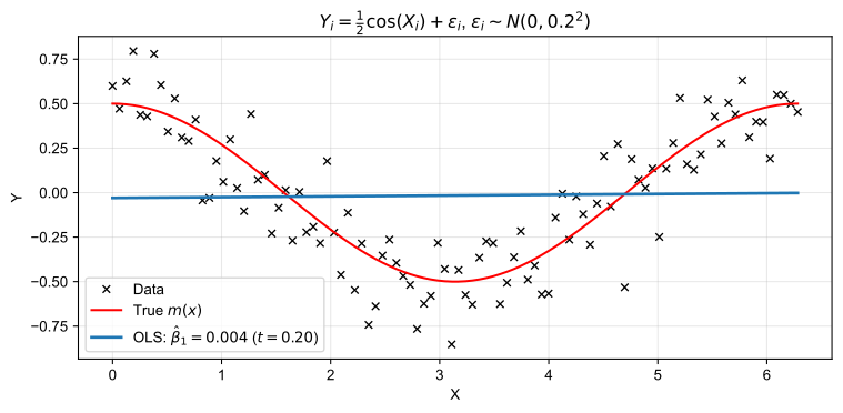
What if \(X\) is discrete?

• Assume that \(X \in \{x_1, x_2, \dots, x_l\}\) for some \(l\). What’s the natural estimator?

\[ \hat{m}(x) = \frac{\sum_{i=1}^{n} I_{\{X_i = x\}}\cdot Y_i}{\sum_{i=1}^n I_{\{X_i = x\}}} \]

• Example: binary \(X\), a treatment
• Exercise: show that this estimator is consistent under mild conditions
• How would you describe this estimator in words?

What about the continuous case?

• Now assume \(X \in \R \implies\) the event \(\{X_i = x\}\) has zero probability
• Well… if \(m(\cdot)\) is continuous, observing points in a neighborhood of \(x\) might be good enough!
• Problem: how large is a neighborhood?

Given \(h>0\) (the bandwidth), the binned estimator is \[ \hat{m}(x) = \frac{ \displaystyle\sum_{i=1}^n I_{\left\{ |X_i - x| \leq h \right\}}\cdot Y_i }{ \displaystyle\sum_{i=1}^n I_{\left\{ |X_i - x| \leq h \right\}} } \]

• What role does \(h\) play here? Small vs large \(h\)?

The Binned Estimator as a Weighted Average

We can also write \[ \hat{m}(x) = \sum_{i=1}^n w_i(x)\cdot Y_i, \qquad w_i(x) \equiv \frac{I_{\left\{ |X_i - x| \leq h \right\}}}{\sum_{j=1}^n I_{\left\{ |X_j - x| \leq h \right\}}} \] where the \(w_i(x)\)’s are weakly positive and \(\sum_{i=1}^n w_i(x) = 1\).

• This estimator is a weighted average of the \(Y_i\)’s, with \(x\)-dependent weights
• True or false: can we interpret these weights as a probability distribution?

• How do these weights change with \(h\)? Smoothly? Sharply?

• One important drawback: the weights change discontinuously with \(h\)!
• \(\hat{m}(x)\) is always a step function, even if \(m(\cdot)\) is continuous!

Kernels

Kernels

• Ideally: points close to \(x\) should matter more for estimation, in a smooth way
• We would like a “continuous way” of measuring distances
• (Continuous) kernels are exactly what we need: they are fancy weights

Definition (Second-Order Kernel)

A second-order kernel function \(K(u)\) satisfies:

1. \(0 \leq K(u) \leq \bar{K} < \infty\) \(\implies\) the kernel is non-negative and bounded
2. \(K(u) = K(-u)\) \(\implies\) the kernel is symmetric around zero
3. \(\int_{-\infty}^{\infty} K(u)\,du = 1\) \(\implies\) like asking the weights to sum to 1
4. \(\int_{-\infty}^{\infty}|u|^r K(u)\,du < \infty\) for positive integers \(r\) \(\implies\) “not too fat tails”

Examples

Kernel	Formula	\(R(K)\)
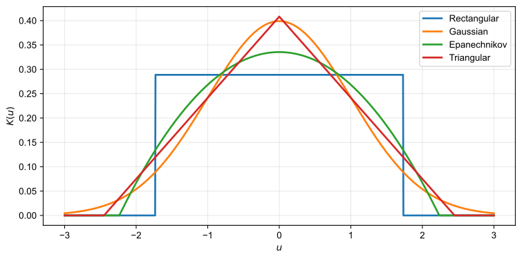
Rectangular	\(\displaystyle K(u) = \begin{cases} \dfrac{1}{2\sqrt{3}} & \text{if } \lvert u\rvert < \sqrt{3} \\ 0 & \text{otherwise} \end{cases}\)	\(\displaystyle \dfrac{1}{2\sqrt{3}}\)
Gaussian	\(\displaystyle K(u) = \frac{1}{\sqrt{2\pi}}\exp\left(-\frac{u^2}{2}\right)\)	\(\displaystyle \frac{1}{2\sqrt{\pi}}\)
Epanechnikov	\(\displaystyle K(u) = \begin{cases} \dfrac{3}{4\sqrt{5}}\left(1-\dfrac{u^2}{5}\right) & \text{if } \lvert u\rvert < \sqrt{5} \\ 0 & \text{otherwise} \end{cases}\)	\(\displaystyle \dfrac{3\sqrt{5}}{25}\)
Triangular	\(\displaystyle K(u) = \begin{cases} \dfrac{1}{\sqrt{6}}\left(1-\dfrac{\lvert u\rvert}{\sqrt{6}}\right) & \text{if } \lvert u\rvert < \sqrt{6} \\ 0 & \text{otherwise} \end{cases}\)	\(\displaystyle \dfrac{\sqrt{6}}{9}\)

All four are scaled to have unit variance. \(R(K) \equiv \int K(u)^2\,du\) is the kernel’s roughness (more on it later).

What Do They Look Like?

A More General Estimator

For a given bandwidth \(h>0\), the Nadaraya-Watson (NW) estimator is \[ \hat{m}(x) = \frac{\sum_{i=1}^n K\left(\frac{X_i - x}{h}\right) \cdot Y_i}{\sum_{i=1}^n K\left(\frac{X_i - x}{h}\right)} \]

• Common choices of kernel: Gaussian and Epanechnikov
• Choosing the bandwidth matters more than choosing the kernel

• What happens when \(h \rightarrow 0\)? And when \(h \rightarrow \infty\)?

• Exercise: which kernel gives back the binned estimator?

Pick Your Own \(h\) and \(n\)

viewof h = Inputs.range([0.02, 3], {value: 0.3, step: 0.01, transform: Math.log, label: "Bandwidth h"})
viewof n = Inputs.range([20, 5000], {value: 100, step: 1, transform: Math.log, label: "Sample size n"})
viewof kernel = Inputs.radio(["Gaussian", "Epanechnikov"], {value: "Gaussian", label: "Kernel"})

data = d3.range(n).map(i => {
  const x = 2 * Math.PI * i / (n - 1)
  const m = 0.5 * Math.cos(x)
  return {x, m, y: m + eps_pool[i]}
})

// Unit-variance kernels, as in the table (normalizing constants cancel in NW)
K = kernel === "Gaussian"
  ? (u => Math.exp(-0.5 * u * u))
  : (u => Math.abs(u) < Math.sqrt(5) ? 1 - u * u / 5 : 0)

// Nadaraya-Watson on a grid; 0/0 (no data in the window) leaves a gap
fit = d3.range(301).map(j => {
  const x0 = 2 * Math.PI * j / 300
  let num = 0, den = 0
  for (const d of data) { const w = K((d.x - x0) / h); num += w * d.y; den += w }
  return {x: x0, mhat: den > 0 ? num / den : NaN}
})

Plot.plot({
  width: 1200, height: 430, marginLeft: 60, marginBottom: 50,
  style: {fontSize: "21px", fontFamily: "Arial, Arimo, sans-serif"},
  x: {label: "X", labelAnchor: "center", labelArrow: "none"},
  y: {label: null, domain: [-1, 1], ticks: 5},
  grid: true,
  marks: [
    Plot.dot(data, {x: "x", y: "y", symbol: "times", stroke: "black",
             r: n <= 200 ? 4 : n <= 1000 ? 3 : 2, strokeOpacity: n <= 200 ? 1 : n <= 1000 ? 0.6 : 0.35}),
    Plot.line(data, {x: "x", y: "m", stroke: "#C62828", strokeWidth: 2, strokeDasharray: "7,5"}),
    Plot.line(fit, {x: "x", y: "mhat", stroke: "#0072BC", strokeWidth: 3}),
    Plot.text([`NW fit, h = ${h.toFixed(2)}, n = ${n}`], {frameAnchor: "bottom-right", dx: -10, dy: -38, fill: "#0072BC", fontWeight: "bold", fontSize: 22, stroke: "white", strokeWidth: 6}),
    Plot.text(["true m(x)"], {frameAnchor: "bottom-right", dx: -10, dy: -10, fill: "#C62828", fontSize: 22, stroke: "white", strokeWidth: 6})
  ]
})

 

Questions?

Asymptotic Properties

Does It Work?

• Do we have any guarantees that this methodology works?
• Yes, but flexibility comes with many caveats! Focus on the intuition

Asymptotic setup:

• The sample size \(n \rightarrow \infty\)
• We also need \(h = h(n)\) to converge to zero \(\implies h \rightarrow 0\)
• But not too fast \(\implies n h \rightarrow \infty\)
• Is this intuitive? Why?

• The asymptotic theory is pointwise, i.e., for a fixed value of \(x\)
• The asymptotic distribution of our estimator changes as \(x\) changes
• Very important: we work through the case of an interior point \(x\)

Asymptotic Theory

Write \(Y_i = m(X_i) + U_i\), where \(\E[U_i|X_i] = 0\) and \(\sigma^2(x) \equiv \Var(U_i | X_i = x)\).

Fix \(x \in \R\) and write \(Y_i = m(x) + \left(m(X_i) - m(x)\right) + U_i\).

Then: \[ \begin{aligned} \frac{1}{nh} \sum_{i=1}^n K\left( \frac{X_i - x}{h} \right) Y_i &= \frac{1}{nh} \sum_{i=1}^n K\left( \frac{X_i - x}{h} \right) m(x) \\ &\quad + \underbrace{\frac{1}{nh} \sum_{i=1}^n K\left( \frac{X_i - x}{h} \right) \left(m(X_i) - m(x)\right)}_{\equiv\, \hat{\Delta}_1(x)} \\ &\quad + \underbrace{\frac{1}{nh} \sum_{i=1}^n K\left( \frac{X_i - x}{h} \right) U_i}_{\equiv\, \hat{\Delta}_2(x)} \end{aligned} \]

Asymptotic Theory

• Assume \(X\) has density \(f(\cdot)\), with \(f(x) > 0\)
• Let \(f_n(x) \equiv \frac{1}{nh} \sum_{i=1}^n K\left( \frac{X_i - x}{h} \right)\)
• This is the non-parametric kernel density estimator: a fancy histogram
• Exercise (problem set): show that \(f_n(x) \xrightarrow{p} f(x)\) as \(n\rightarrow \infty\)
• For now, we take this result for granted

• Dividing the previous expression by \(f_n(x)\):

\[ \hat{m}(x) - m(x) = \frac{1}{f_n(x)}\left[\hat{\Delta}_1(x) + \hat{\Delta}_2(x) \right] \]

Asymptotic Theory

We will show that \(\sqrt{nh}\cdot \hat{\Delta}_1(x)\) converges in probability and \(\sqrt{nh}\cdot \hat{\Delta}_2(x)\) has a limiting distribution.

• First, \(\hat{\Delta}_2(x)\). Notice that \[ \E\left[ \frac{1}{nh} \sum_{i=1}^n K\left( \frac{X_i - x}{h} \right) U_i \right] = \frac{1}{h} \E\left[K\left( \frac{X_i - x}{h} \right) U_i\right] = 0 \]

• We also see that \[ \begin{aligned} \Var\left[ \hat{\Delta}_2(x) \right] &= \frac{1}{nh^2} \E \left[ \left( K\left( \frac{X_i - x}{h} \right) U_i \right)^2 \right] = \frac{1}{nh^2} \E \left[ K\left( \frac{X_i - x}{h} \right)^2 \sigma^2(X_i) \right] \\ &= \frac{1}{nh^2} \int_{-\infty}^{\infty} K\left( \frac{z - x}{h} \right)^2 \sigma^2(z) f(z) \, dz \end{aligned} \]

Asymptotic Theory

• Change variables: \(u = \frac{z-x}{h}\)
• We can only do this because \(x\) is in the interior of its support
• The last integral becomes

\[ \frac{1}{nh^2} \int_{-\infty}^{\infty} K\left( \frac{z - x}{h} \right)^2 \sigma^2(z) f(z) \, dz = \frac{1}{nh} \int_{-\infty}^{\infty} K(u)^2\, \sigma^2(x + hu)\, f(x + hu)\, du \]

• Assume that \(\sigma^2(\cdot)\) and \(f(\cdot)\) are continuous
• For any continuous \(g(\cdot)\) and fixed \(u\): \(g(x + hu) = g(x) + o(1)\) as \(h\rightarrow 0\)

\[ \frac{1}{nh} \int_{-\infty}^{\infty} K(u)^2\, \sigma^2(x + hu)\, f(x + hu)\, du = \frac{\sigma^2(x)f(x)}{nh}\int_{-\infty}^{\infty}K(u)^2\,du + o\left(\frac{1}{nh}\right) \]

Asymptotic Theory

• Define \(R(K)\equiv \int_{-\infty}^{\infty}K(u)^2\,du\), the roughness of the kernel
• We have shown that

\[ \Var\left[ \hat{\Delta}_2(x) \right] = \frac{\sigma^2(x)f(x)R(K)}{nh} + o\left(\frac{1}{nh}\right) \]

• Important: the variance of this term only vanishes if \(nh \rightarrow \infty\)
• Fast \(h \rightarrow 0 \implies\) slow convergence of this variance to zero
• By the Lindeberg-Feller CLT:

\[ \sqrt{nh}\,\hat{\Delta}_2(x) \xrightarrow{d} N\left(0, \sigma^2(x)f(x)R(K)\right) \]

• Notice how the asymptotic variance depends on \(x\)!

Asymptotic Theory

Now the other guy, \(\hat{\Delta}_1(x)\), using similar tricks: \[ \begin{aligned} \E[\hat{\Delta}_1(x)] &= \frac{1}{h} \, \E \left[ K\left( \frac{X_i - x}{h} \right) \left( m(X_i) - m(x) \right) \right] \\ &= \frac{1}{h} \int_{-\infty}^{\infty} K\left( \frac{z - x}{h} \right) \left( m(z) - m(x) \right) f(z) \, dz \\ &= \int_{-\infty}^{\infty} K(u) \left( m(x + hu) - m(x) \right) f(x + hu) \, du \end{aligned} \]

Add the assumptions \(f \in C^1\) and \(m \in C^2\), and expand: \[ \begin{gathered} m(x + hu) - m(x) = m'(x)hu + \tfrac{1}{2} m''(x) h^2 u^2 + o(h^2)\\ f(x + hu) = f(x) + f'(x)hu + o(h) \end{gathered} \]

Asymptotic Theory

Distribute the terms:

\[ (m(x + hu) - m(x)) \cdot f(x + hu) = m'(x)f(x)hu + m'(x)f'(x)h^2u^2 + \tfrac{1}{2}m''(x)f(x)h^2u^2 + o(h^2) \]

The term linear in \(u\) integrates to zero (symmetric \(K\)), so: \[ \begin{aligned} \E[\hat{\Delta}_1(x)] &= h^2 \left(\int_{-\infty}^{\infty}u^2K(u)\,du\right)\left(m'(x)f'(x) + \tfrac{1}{2}m''(x)f(x)\right) + o(h^2)\\ & = h^2 \kappa_2 f(x) B(x) + o(h^2) \end{aligned} \] where \(B(x) \equiv m'(x)\frac{f'(x)}{f(x)} + \frac{1}{2}m''(x)\) and \(\kappa_2\equiv \int_{-\infty}^{\infty}u^2K(u)\,du\).

Questions: is \(B(x)\) random? How does \(h\) affect \(\E[\hat{\Delta}_1(x)]\)?

Asymptotic Theory

• Computing \(\Var(\hat{\Delta}_1(x))\) is boring
• See Section 19.26 in Hansen’s Econometrics. He shows that

\[ \Var(\hat{\Delta}_1(x)) = o\left(\frac{1}{nh}\right) \]

• This implies \(\Var(\sqrt{nh}\,\hat{\Delta}_1(x)) = o(1)\)
• The main result is that

\[ \sqrt{nh}\left(\hat{\Delta}_1(x) - h^2 \kappa_2 f(x) B(x)\right) \xrightarrow{p} 0 \]

as long as \(nh^5 = O(1)\) (why do we need this?)

Asymptotic Theory: Main Result

See Chapter 19 of Hansen’s Econometrics for all the technical conditions.

Theorem (Asymptotic Distribution of the NW Estimator)

Under regularity conditions, for interior \(x\), \[ \sqrt{nh} \left( \hat{m}(x) - m(x) - h^2 \kappa_2 B(x) \right) \xrightarrow{d} N\left(0, \frac{\sigma^2(x) R(K)}{f(x)} \right) \] where \(B(x) = m'(x)\frac{f'(x)}{f(x)} + \frac{1}{2}m''(x)\).

• Why is the convergence rate \(\sqrt{nh}\) and not just \(\sqrt{n}\)?
• True or false: is there always a finite-sample bias here?

 

Questions?

Implementation Matters

The Bias-Variance Trade-off

• If \(n\) is very large:

\[ \hat{m}(x) - m(x) \approx N\left(h^2 \kappa_2 B(x), \frac{\sigma^2(x)R(K)}{nh\cdot f(x)}\right) \]

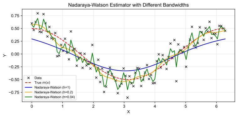
• What is the effect of \(h\) on the mean and on the variance?

• Fundamental trade-off: we can reduce the bias at the expense of variance
• Or you can get low variance… and a huge bias!

• The Epanechnikov kernel minimizes the mean squared error of this estimator across a large class of kernels
• The efficiency loss from the Gaussian kernel is minimal
• Honestly, let the Gaussian kernel be your default in empirical research

How to Pick the Bandwidth?

• The optimal bandwidth depends on moments of the data and derivatives of \(m\)
• Those are unknown in practice
• Ideally, your results should be robust to different bandwidths (within reason)
• A popular way to choose a bandwidth: leave-one-out cross-validation
• Exactly what the Machine Learning literature does!
• See Hansen’s Econometrics for details and the theory behind it

Different Bandwidths

What About the Boundary?

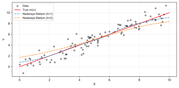
• Suppose \(X_i\) comes from a bounded distribution
• Say \(X \sim U[0,10]\) and \(Y|X = x \sim N(x, 1)\)

The Local Linear Estimator

• The Nadaraya-Watson estimator also solves

\[ \hat{m}(x) = \arg\min_{c \in \R} \sum_{i=1}^{n}K\left(\frac{X_i - x}{h}\right)\cdot (Y_i-c)^2 \]

• That’s why it’s also called the local-constant estimator

• What is stopping us from fitting a linear function here?

Definition (Local-Linear Estimator)

For each \(x\), solve \[ \left(\hat{\beta}_0(x), \hat{\beta}_1(x)\right) = \arg \min_{(b_0, b_1)} \sum_{i=1}^n K\left(\frac{X_i - x}{h}\right)(Y_i - b_0 - b_1(X_i - x))^2 \] The local-linear estimator of \(m(x)\), denoted \(\hat{m}_{LL}(x)\), is the local intercept \(\hat{\beta}_0(x)\).

How Do They Compare?

• Deriving the asymptotic distribution requires similar tricks (see Hansen’s Econometrics)
• Important: both have the same asymptotic variance
• Also important: the bias term of the local-linear estimator is \(h^2 \kappa_2 \frac{m''(x)}{2}\)

\[ \sqrt{nh} \left( \hat{m}_{LL}(x) - m(x) - h^2 \kappa_2 \frac{m''(x)}{2} \right) \xrightarrow{d} N\left(0, \frac{\sigma^2(x) R(K)}{f(x)} \right) \]

• What does this imply if \(m(\cdot)\) is, in fact, linear?
• The local-linear estimator is much better close to the boundary! Why?

Back to the Boundary

• Same data as before: \(X \sim U[0,10]\) and \(Y|X = x \sim N(x, 1)\)

viewof h_bd = Inputs.range([0.2, 5], {value: 1, step: 0.01, transform: Math.log, label: "Bandwidth h"})

fit_bd = d3.range(201).map(j => {
  const x0 = 10 * j / 200
  let S0 = 0, S1 = 0, S2 = 0, T0 = 0, T1 = 0
  for (let i = 0; i < X_bd.length; i++) {
    const d = X_bd[i] - x0, u = d / h_bd, w = Math.exp(-0.5 * u * u)
    S0 += w; S1 += w * d; S2 += w * d * d; T0 += w * Y_bd[i]; T1 += w * d * Y_bd[i]
  }
  return {x: x0, nw: T0 / S0, ll: (S2 * T0 - S1 * T1) / (S0 * S2 - S1 * S1)}
})

Plot.plot({
  width: 1200, height: 470, marginLeft: 60, marginBottom: 50,
  style: {fontSize: "21px", fontFamily: "Arial, Arimo, sans-serif"},
  x: {label: "X", labelAnchor: "center", labelArrow: "none", domain: [0, 10]},
  y: {label: null, domain: [-2, 12], ticks: 5},
  grid: true,
  marks: [
    Plot.dot(X_bd.map((x, i) => ({x, y: Y_bd[i]})), {x: "x", y: "y", stroke: "black", r: 4, clip: true}),
    Plot.line([{x: 0}, {x: 10}], {x: "x", y: "x", stroke: "#C62828", strokeWidth: 2, strokeDasharray: "7,5"}),
    Plot.line(fit_bd, {x: "x", y: "nw", stroke: "#0072BC", strokeWidth: 3, clip: true}),
    Plot.line(fit_bd, {x: "x", y: "ll", stroke: "#EB811B", strokeWidth: 3, clip: true}),
    Plot.text([`Nadaraya-Watson, h = ${h_bd.toFixed(2)}`], {frameAnchor: "bottom-right", dx: -10, dy: -66, fill: "#0072BC", fontWeight: "bold", fontSize: 22, stroke: "white", strokeWidth: 6}),
    Plot.text([`Local linear, h = ${h_bd.toFixed(2)}`], {frameAnchor: "bottom-right", dx: -10, dy: -38, fill: "#EB811B", fontWeight: "bold", fontSize: 22, stroke: "white", strokeWidth: 6}),
    Plot.text(["true m(x)"], {frameAnchor: "bottom-right", dx: -10, dy: -10, fill: "#C62828", fontSize: 22, stroke: "white", strokeWidth: 6})
  ]
})

 

Questions?

Curse of Dimensionality

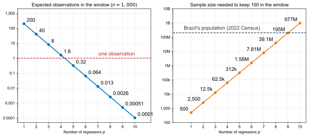
• So far, \(x\) was a scalar. What if \(X_i \in \R^p\) with \(p >1\)?
• Use multivariate kernels and measure “distances” to \(x = (x_1, \dots, x_p)\) as \[ K\left(\frac{X_{i1} - x_1}{h_1}\right)\cdot K\left(\frac{X_{i2} - x_2}{h_2}\right) \cdots K\left(\frac{X_{ip} - x_p}{h_p}\right) \] where \((h_1, \dots, h_p)\) are potentially different bandwidths
• The math gets more involved, but we get the same type of results

• Super important caveat: convergence happens at rate \(\sqrt{n\cdot h_1\cdot h_2 \cdots h_p}\)
• With a common \(h\), we need \(nh^p \rightarrow \infty\). This is very slow
• In practice, if \(p > 4\) you are screwed \(\implies\) open the Machine Learning toolbox

How Fast Does the Neighborhood Empty Out?

\(X \sim U[0,1]^p\), window of half-width \(h = 0.1\): it covers a share \(0.2^p\) of the cube

Confidence Bands

• You did all the math to get the distribution, so you might want to make inference about \(m(x)\)…
• Keep in mind: any confidence band you draw is pointwise
• Usually, we cheat and compute the 95% confidence interval as

\[ \hat{m}(x) \pm 1.96 \cdot \sqrt{\frac{\hat{\sigma}^2(x) R(K)}{nh\, f_n(x)}} \]

where \(\hat{\sigma}^2(x)\) comes from the residuals of your fit, smoothed with the same kernel

• Why is this cheating?

Confidence Bands in Action

viewof n_ci = Inputs.range([20, 5000], {value: 100, step: 1, transform: Math.log, label: "Sample size n"})
viewof h_ci = Inputs.range([0.05, 1.5], {value: 0.3, step: 0.01, transform: Math.log, label: "Bandwidth h"})

band = {
  const n = n_ci, h = h_ci, dx = 2 * Math.PI / (n - 1)
  const RK = 1 / (2 * Math.sqrt(Math.PI))  // R(K) for the Gaussian kernel
  const X = d3.range(n).map(i => i * dx)
  const Y = X.map((x, i) => 0.5 * Math.cos(x) + eps_pool[i])

  // Kernel-weighted average of v at x0 (skipping observation `skip`), and
  // sum_i K((X_i - x0)/h) = n h f_n(x0). X is an even grid, so only visit |u| < 6.
  const smooth = (v, x0, skip = -1) => {
    const lo = Math.max(0, Math.ceil((x0 - 6 * h) / dx))
    const hi = Math.min(n - 1, Math.floor((x0 + 6 * h) / dx))
    let num = 0, den = 0
    for (let i = lo; i <= hi; i++) {
      if (i === skip) continue
      const u = (X[i] - x0) / h, w = Math.exp(-0.5 * u * u)
      num += w * v[i]; den += w
    }
    return {avg: num / den, sumK: den / Math.sqrt(2 * Math.PI)}
  }

  // Squared leave-one-out residuals, smoothed with the same kernel give sigma^2(x)
  const e2 = X.map((x, i) => (Y[i] - smooth(Y, x, i).avg) ** 2)
  const fit = d3.range(301).map(j => {
    const x = 2 * Math.PI * j / 300
    const {avg: mhat, sumK} = smooth(Y, x)
    const se = Math.sqrt(smooth(e2, x).avg * RK / sumK)
    return {x, m: 0.5 * Math.cos(x), mhat, lo: mhat - 1.96 * se, hi: mhat + 1.96 * se}
  })
  const ok = fit.filter(d => d.lo <= d.m && d.m <= d.hi).length
  return {data: X.map((x, i) => ({x, y: Y[i]})), fit, cover: ok / fit.length}
}

Plot.plot({
  width: 1200, height: 450, marginLeft: 60, marginBottom: 50,
  style: {fontSize: "21px", fontFamily: "Arial, Arimo, sans-serif"},
  x: {label: "X", labelAnchor: "center", labelArrow: "none"},
  y: {label: null, domain: [-1, 1], ticks: 5},
  grid: true,
  marks: [
    Plot.dot(band.data, {x: "x", y: "y", symbol: "times", stroke: "black", clip: true,
             r: n_ci <= 200 ? 4 : n_ci <= 1000 ? 3 : 2, strokeOpacity: n_ci <= 200 ? 1 : n_ci <= 1000 ? 0.6 : 0.35}),
    Plot.areaY(band.fit, {x: "x", y1: "lo", y2: "hi", fill: "#0072BC", fillOpacity: 0.25, clip: true}),
    Plot.line(band.fit, {x: "x", y: "m", stroke: "#C62828", strokeWidth: 2, strokeDasharray: "7,5"}),
    Plot.line(band.fit, {x: "x", y: "mhat", stroke: "#0072BC", strokeWidth: 3, clip: true}),
    Plot.text([`NW fit + 95% band, h = ${h_ci.toFixed(2)}, n = ${n_ci}`], {frameAnchor: "bottom-right", dx: -10, dy: -66, fill: "#0072BC", fontWeight: "bold", fontSize: 22, stroke: "white", strokeWidth: 6}),
    Plot.text(["true m(x)"], {frameAnchor: "bottom-right", dx: -10, dy: -38, fill: "#C62828", fontSize: 22, stroke: "white", strokeWidth: 6}),
    Plot.text([`band covers m(x) at ${Math.round(100 * band.cover)}% of points`], {frameAnchor: "bottom-right", dx: -10, dy: -10, fill: "#EB811B", fontWeight: "bold", fontSize: 22, stroke: "white", strokeWidth: 6})
  ]
})

 

Questions?

References

• Chapter 19 of Econometrics, by Bruce Hansen
• Chapter 17 of Probability and Statistics for Economists, by Bruce Hansen